
In mechanical engineering, screw gears, commonly known as worm drives, play a pivotal role in transmitting motion and power between non-intersecting shafts, typically at right angles. These screw gears offer significant advantages, including high reduction ratios, compact design, smooth operation, and low noise, making them indispensable in industries such as mining, metallurgy, and transportation. However, traditional design methods for screw gears often rely on empirical rules and iterative trial-and-error approaches, which can be time-consuming and may not yield optimal solutions. To address the inherent drawbacks of high cost and low efficiency in conventional cylindrical screw gear systems, this paper presents a comprehensive multi-objective fuzzy optimization framework. Leveraging fuzzy set theory and Matlab’s computational capabilities, I aim to minimize the volume of the worm wheel rim and maximize transmission efficiency simultaneously. The proposed methodology not only enhances design precision but also provides a robust tool for engineers seeking to improve screw gear performance. Throughout this discussion, the term “screw gears” will be emphasized to underscore their helical engagement mechanism, which is central to this optimization endeavor.
The core of this work lies in formulating a fuzzy optimization model that accounts for the inherent uncertainties in design parameters and constraints. Unlike classical optimization, fuzzy optimization incorporates vagueness in engineering specifications, allowing for a more realistic representation of design goals. I begin by establishing the mathematical model, defining design variables, objective functions, and constraints. Subsequently, I introduce fuzzy membership functions to handle imprecise boundaries and perform defuzzification to convert the fuzzy model into a crisp one. Finally, I implement the optimization using Matlab programming and its Optimization Toolbox, demonstrating significant improvements in volume reduction and efficiency enhancement. This approach is particularly relevant for screw gears, where material cost and energy loss are critical concerns. By integrating fuzzy logic with numerical optimization, I offer a novel perspective on screw gear design that balances multiple conflicting objectives effectively.
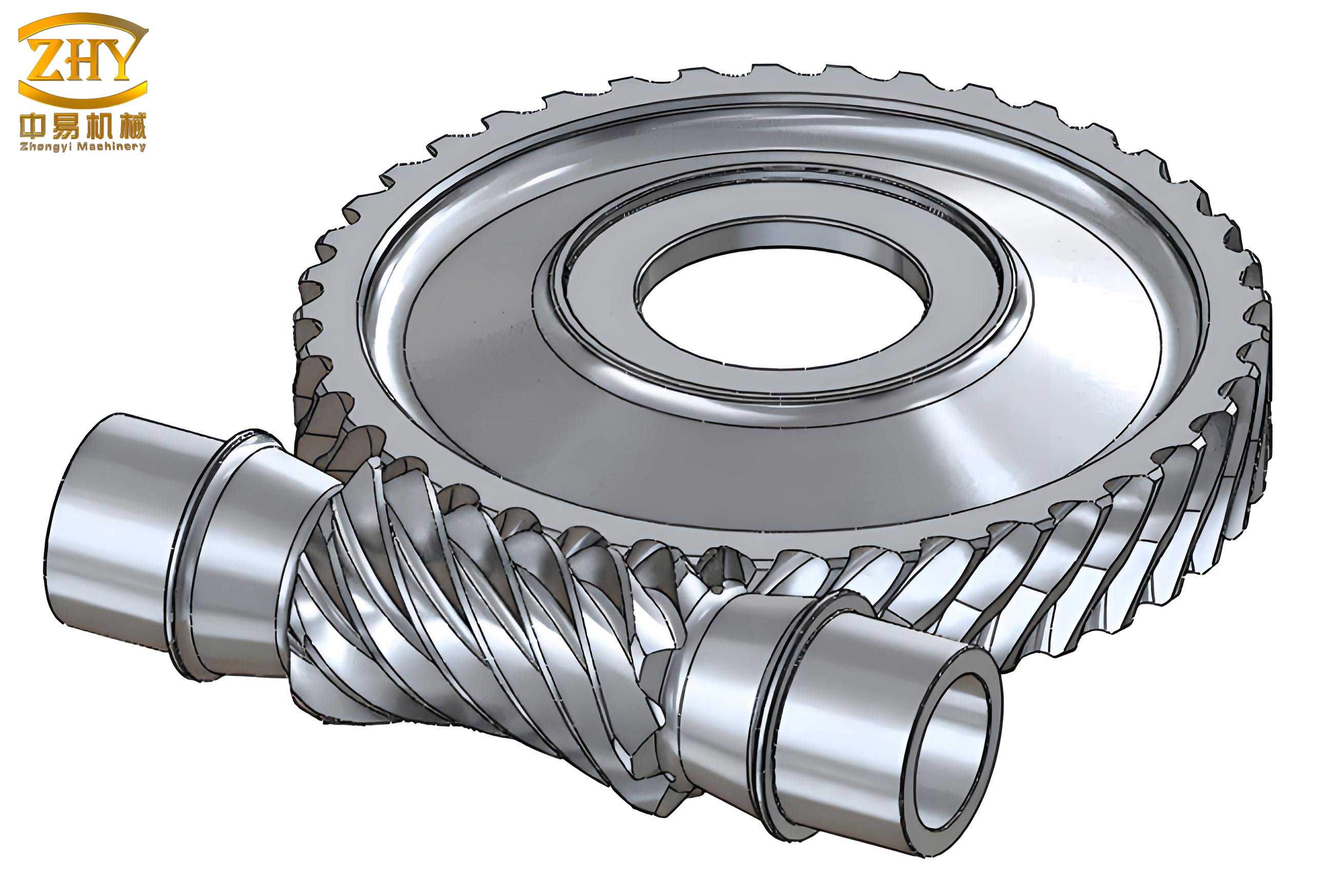
To illustrate the practical application, consider a typical screw gear system with a transmission ratio of 20, input power of 7.5 kW, and input speed of 960 rpm. The worm is made of steel, while the worm wheel is crafted from tin bronze, a common material pairing for screw gears due to its wear resistance. The goal is to optimize the geometric parameters to reduce material usage and improve efficiency, which directly impacts operational costs and sustainability. In the following sections, I delve into the detailed mathematical formulation, fuzzy processing, and computational implementation, supported by tables and equations to clarify each step. The use of screw gears in heavy-duty applications necessitates such advanced design techniques to ensure reliability and performance under varying loads.
Fuzzy Optimization Mathematical Model for Screw Gears
The fuzzy optimization model for screw gears is built upon the foundation of classical optimization but extends it to accommodate fuzzy constraints and objectives. This model captures the designer’s experience and tolerance ranges, making it more adaptive to real-world scenarios. I define the model in three parts: design variables, objective functions, and constraints. Each component is critical for accurately representing the screw gear system and achieving the desired optimization outcomes.
Design Variables
In screw gear design, several parameters influence performance, but for optimization, I select independent variables that significantly affect the objectives and are controllable during design. The key variables are the number of worm threads (z₁), module (m), and diameter factor (q). These parameters directly impact the gear’s size, strength, and efficiency. Thus, the design vector is expressed as:
$$ \mathbf{X} = [x_1, x_2, x_3]^T = [z_1, m, q]^T $$
Here, \(x_1\) represents the worm thread count, \(x_2\) the module, and \(x_3\) the diameter factor. These variables form the basis for optimizing screw gears, as they dictate the geometric and kinematic properties. For instance, the worm thread count affects the lead angle and efficiency, while the module influences tooth size and load capacity. The diameter factor balances rigidity and manufacturability. By optimizing these variables, I aim to achieve a balanced design that meets multiple criteria. The selection of these variables is consistent with standard screw gear design practices, ensuring practicality and applicability.
To provide a clearer overview, Table 1 summarizes the design variables, their symbols, and typical ranges for screw gears in power transmission applications. These ranges will later be incorporated as fuzzy constraints to account for design flexibility.
| Variable | Symbol | Typical Range | Description |
|---|---|---|---|
| Worm threads | \(z_1\) | 2 to 6 | Number of starts on the worm |
| Module | \(m\) | 2 mm to 18 mm | Size of gear teeth |
| Diameter factor | \(q\) | 8 to 15 | Ratio of pitch diameter to module |
Objective Functions
The optimization aims to achieve two primary goals: minimizing the volume of the worm wheel rim to reduce material cost and maximizing transmission efficiency to enhance energy savings. These objectives often conflict; for example, a larger gear may improve strength but increase volume. Therefore, I formulate separate objective functions and then combine them into a unified target using weighting coefficients.
1. Minimizing Worm Wheel Rim Volume: The worm wheel rim, typically made of expensive bronze, contributes significantly to material cost. Minimizing its volume reduces material usage without compromising functionality. The volume \(V\) of the rim is derived from its geometry:
$$ V = \frac{\pi}{4} (d_e^2 – d_0^2) B $$
where \(d_e\) is the maximum rim diameter, \(d_0\) is the minimum rim diameter, and \(B\) is the rim width. For screw gears, these dimensions are expressed in terms of design variables:
$$ d_e = m(i z_1 + 3), \quad d_0 = m(i z_1 – 6.4), \quad B = 0.67 m(q + 2) $$
Here, \(i = 20\) is the transmission ratio. Substituting these into the volume equation yields the first objective function \(f_1(\mathbf{X})\):
$$ f_1(\mathbf{X}) = 0.5262 \, x_2^3 (x_3 + 2) \left[ (20 x_1 + 3)^2 – (20 x_1 – 6.4)^2 \right] $$
This function represents the rim volume in cubic millimeters, and minimization directly correlates with cost reduction for screw gears.
2. Maximizing Transmission Efficiency: Screw gears are prone to high friction losses due to sliding contact, leading to efficiencies typically between 0.75 and 0.92. Improving efficiency is crucial for energy conservation. I express efficiency \(\eta\) as:
$$ \eta = 0.96 \frac{\tan \lambda}{\tan(\lambda + \rho_v)} $$
where \(\lambda\) is the lead angle, \(\tan \lambda = z_1 / q\), and \(\rho_v\) is the equivalent friction angle, dependent on the sliding velocity \(v_s\). The sliding velocity is given by:
$$ v_s = \frac{\pi m n_1}{60 \times 1000} \sqrt{z_1^2 + q^2} \approx \frac{m n_1}{19100} \sqrt{z_1^2 + q^2} $$
with \(n_1 = 960 \, \text{rpm}\). The equivalent friction coefficient \(f_v\) is derived from empirical data using curve fitting in Matlab:
$$ f_v = 0.0175192 e^{1.0460682 / v_s} $$
Thus, \(\tan \rho_v = f_v\). To maximize efficiency, I minimize its reciprocal, leading to the second objective function \(f_2(\mathbf{X})\):
$$ f_2(\mathbf{X}) = \frac{1}{\eta} = \frac{\tan(\lambda + \rho_v)}{0.96 \tan \lambda} = \frac{x_1 x_3 + f_v x_3^2}{0.96 x_1 x_3 – 0.96 x_1^2 f_v} $$
This formulation emphasizes the efficiency aspect of screw gears, which is vital for sustainable design.
3. Unified Objective Function: To handle multiple objectives, I employ a weighted sum approach, combining \(f_1(\mathbf{X})\) and \(f_2(\mathbf{X})\) into a single function. Given that volume is in the order of \(10^6 \, \text{mm}^3\) and efficiency is dimensionless, I scale \(f_2(\mathbf{X})\) by \(10^6\) to align magnitudes. Weighting coefficients \(\omega_1 = 0.8\) and \(\omega_2 = 0.2\) reflect the relative importance of volume reduction versus efficiency improvement, based on engineering priorities for screw gears. The unified objective function \(f(\mathbf{X})\) is:
$$ f(\mathbf{X}) = 0.8 f_1(\mathbf{X}) + 0.2 \times 10^6 f_2(\mathbf{X}) $$
Substituting the expressions:
$$ f(\mathbf{X}) = 0.420976 \, x_2^3 (x_3 + 2) \left[ (20 x_1 + 3)^2 – (20 x_1 – 6.4)^2 \right] – \frac{4.8 \times 10^6 (x_1 x_3 + f_v x_3^2)}{x_1 (x_3 – x_1 f_v)} $$
Minimizing \(f(\mathbf{X})\) achieves a compromise between the two goals, ensuring an optimal balance for screw gear systems.
Constraint Conditions
Constraints ensure the screw gear design meets functional, geometric, and performance requirements. I categorize them into boundary constraints (hard limits on variables) and performance constraints (fuzzy limits based on operational conditions). These constraints are derived from design standards and practical considerations for screw gears.
A. Boundary Constraints: These define the feasible ranges for design variables, based on typical screw gear specifications:
- Worm threads: \(2 \leq g_1(\mathbf{X}) = x_1 \leq 6\)
- Worm wheel teeth: \(30 \leq g_2(\mathbf{X}) = 20 x_1 \leq 80\) (to avoid undercut and excessive size)
- Module: \(2 \leq g_3(\mathbf{X}) = x_2 \leq 18\) (standard series for power transmission)
- Diameter factor: \(8 \leq g_4(\mathbf{X}) = x_3 \leq 15\) (balances lead angle and rigidity)
These constraints are initially crisp but will be fuzzified to allow gradual transitions at boundaries.
B. Performance Constraints: These ensure the screw gear operates safely under load, with fuzzy limits accounting for uncertainties in material properties and operating conditions.
1. Contact Fatigue Strength: The tooth surface must withstand contact stresses to prevent pitting. The constraint is based on the Hertzian contact stress formula:
$$ \sigma_H = Z_E \sqrt{\frac{9400 T_2 K_A K_V K_\beta}{d_1 d_2^2}} \leq [\sigma_H] $$
where \(Z_E = 155 \, \sqrt{\text{MPa}}\) for steel-bronze pair, \(T_2 = 1268.36 \, \text{N·m}\) is the output torque (assuming initial efficiency 0.85), \(K_A = 1.0\) (application factor), \(K_V = 1.1\) (dynamic factor), \(K_\beta = 1.0\) (load distribution factor), \(d_1 = m q\), and \(d_2 = m i z_1\). The allowable stress \([\sigma_H]\) is fuzzy. Substituting values gives:
$$ g_5(\mathbf{X}) = \frac{28066.176}{\sqrt{x_1^2 x_2^3 x_3}} \leq [\sigma_H] $$
This constraint is critical for screw gears to ensure long-term durability against surface failures.
2. Bending Fatigue Strength: The tooth root must resist bending fatigue to avoid breakage. The constraint uses the Lewis formula adapted for screw gears:
$$ \sigma_F = \frac{666 T_2 K_A K_V K_\beta}{d_1 d_2 m} Y_{Fs} Y_\beta \leq [\sigma_F] $$
Here, \(Y_{Fs}\) is the composite tooth form factor, approximated via curve fitting: \(Y_{Fs} = 2.58 e^{-0.049 x_1}\). \(Y_\beta\) is the lead angle factor: \(Y_\beta = 1 – \lambda/120^\circ\), with \(\lambda = \arctan(x_1/x_3)\). The allowable stress \([\sigma_F]\) is fuzzy. Simplifying yields:
$$ g_6(\mathbf{X}) = \frac{119866.869 e^{-0.049 x_1} \left(1 – \frac{\arctan(x_1/x_3)}{120}\right)}{x_1 x_2^3 x_3} \leq [\sigma_F] $$
This ensures the screw gear teeth have adequate bending strength under transmitted loads.
3. Worm Shaft Deflection: Excessive deflection of the worm shaft can misalign mesh, leading to uneven wear and noise. The deflection \(f\) at the mesh point is limited to a fraction of the module:
$$ f = \frac{\sqrt{F_{r1}^2 + F_{t1}^2}}{48 E I} L^3 \leq [f] = m/50 $$
where \(F_{t1} = 2T_2/(i \eta m q)\), \(F_{r1} = 2T_2 \tan \alpha/(m i z_1)\) with pressure angle \(\alpha = 20^\circ\), \(E = 2.1 \times 10^5 \, \text{MPa}\) for steel, \(I = \pi m^4 (q – 2.4)^4/64\) (area moment of inertia), and \(L = 1.1 m(i z_1 + 2)\) (support span). After substitution:
$$ g_7(\mathbf{X}) = \frac{3.411852 \times 10^{-4} (20 x_1 + 2)^3 \sqrt{(0.36397/x_1)^2 + (1.17647/x_3)^2}}{(x_3 – 2.4)^4 x_2^2} \leq 0.02 x_2 $$
This constraint maintains alignment in screw gears, crucial for smooth operation.
4. Sliding Velocity: High sliding velocity can cause overheating and lubrication failure. The constraint limits \(v_s\) to prevent scoring:
$$ v_s = \frac{m n_1}{19100} \sqrt{z_1^2 + q^2} \leq [v_s] $$
Taking \([v_s] = 16 \, \text{m/s}\) as a fuzzy limit:
$$ g_8(\mathbf{X}) = 0.05026178 \, x_2 \sqrt{x_1^2 + x_3^2} \leq [v_s] $$
This is essential for screw gears to ensure effective lubricant film and avoid seizure.
5. Thermal Balance: Screw gears generate heat due to friction, which must be dissipated to prevent oil degradation. The temperature rise \(\Delta t\) is constrained by:
$$ \Delta t = \frac{1000 P (1 – \eta)}{k_s A} \leq [\Delta t] $$
with \(P = 7.5 \, \text{kW}\), \(k_s = 15 \, \text{W/(m}^2 \cdot \text{°C)}\) (heat transfer coefficient), and \(A = 0.33 \left( \frac{m(q + i z_1)}{200} \right)^{1.75}\) (housing surface area). Assuming \([\Delta t] = 60^\circ \text{C}\):
$$ g_9(\mathbf{X}) = \frac{2417407.226}{[x_2 (x_3 + 20 x_1)]^{1.75}} \leq [\Delta t] $$
This ensures thermal stability for screw gears in continuous operation.
Table 2 summarizes all performance constraints, their mathematical forms, and fuzzy allowable limits, highlighting the multi-faceted nature of screw gear design.
| Constraint | Expression \(g_j(\mathbf{X})\) | Fuzzy Allowable Limit | Purpose |
|---|---|---|---|
| Contact stress | \( \frac{28066.176}{\sqrt{x_1^2 x_2^3 x_3}} \) | \([\sigma_H]\) | Prevent surface pitting |
| Bending stress | \( \frac{119866.869 e^{-0.049 x_1} (1 – \frac{\arctan(x_1/x_3)}{120})}{x_1 x_2^3 x_3} \) | \([\sigma_F]\) | Avoid tooth breakage |
| Shaft deflection | \( \frac{3.411852 \times 10^{-4} (20 x_1 + 2)^3 \sqrt{(0.36397/x_1)^2 + (1.17647/x_3)^2}}{(x_3 – 2.4)^4 x_2^2} \) | \(0.02 x_2\) | Maintain alignment |
| Sliding velocity | \( 0.05026178 \, x_2 \sqrt{x_1^2 + x_3^2} \) | \([v_s]\) | Control lubrication |
| Temperature rise | \( \frac{2417407.226}{[x_2 (x_3 + 20 x_1)]^{1.75}} \) | \([\Delta t]\) | Ensure thermal safety |
Fuzzy Membership Functions and Defuzzification
In real-world screw gear design, constraints often have gradual transitions rather than sharp boundaries. Fuzzy set theory handles this by assigning membership degrees between 0 and 1, indicating how well a design satisfies a constraint. I define linear membership functions for simplicity and practicality, then determine fuzzy allowable intervals using expansion coefficients based on engineering experience.
Membership Functions for Performance Constraints
For each performance constraint \(g_j(\mathbf{X}) \leq \sigma_j\), where \(\sigma_j\) is the fuzzy allowable limit, I define a membership function \(\mu_{g_j}(\mathbf{X})\) that decreases linearly from 1 to 0 over a transition zone. Let \(\sigma_j^l\) and \(\sigma_j^u\) be the lower and upper bounds of the fuzzy interval, respectively. Then:
$$ \mu_{g_j}(\mathbf{X}) =
\begin{cases}
1 & \text{if } g_j(\mathbf{X}) \leq \sigma_j^l \\
\frac{\sigma_j^u – g_j(\mathbf{X})}{\sigma_j^u – \sigma_j^l} & \text{if } \sigma_j^l \leq g_j(\mathbf{X}) \leq \sigma_j^u \\
0 & \text{if } g_j(\mathbf{X}) \geq \sigma_j^u
\end{cases} $$
This function reflects the degree of satisfaction: 1 means fully satisfied, 0 means violated, and intermediate values indicate partial satisfaction. For screw gears, this accounts for uncertainties in material properties and operating conditions.
Membership Functions for Boundary Constraints
Boundary constraints on design variables also exhibit fuzziness. For a variable \(x_j\) with lower bound \(x_j^l\) and upper bound \(x_j^u\), the membership function \(\mu_{x_j}\) is defined piecewise:
$$ \mu_{x_j} =
\begin{cases}
0 & \text{if } x_j \leq x_j^{l-} \\
\frac{x_j – x_j^{l-}}{x_j^{l+} – x_j^{l-}} & \text{if } x_j^{l-} \leq x_j \leq x_j^{l+} \\
1 & \text{if } x_j^{l+} \leq x_j \leq x_j^{u-} \\
\frac{x_j^{u+} – x_j}{x_j^{u+} – x_j^{u-}} & \text{if } x_j^{u-} \leq x_j \leq x_j^{u+} \\
0 & \text{if } x_j \geq x_j^{u+}
\end{cases} $$
Here, \(x_j^{l-}\) and \(x_j^{l+}\) are the lower and upper limits of the lower fuzzy boundary, while \(x_j^{u-}\) and \(x_j^{u+}\) are for the upper fuzzy boundary. This allows smooth transitions at the edges, accommodating design flexibility for screw gears.
Determining Fuzzy Allowable Intervals
I use the expansion coefficient method to set the fuzzy intervals, based on conventional design values. For performance constraints, the lower bound \(\sigma_j^l\) is the conventional allowable value, and the upper bound \(\sigma_j^u\) is expanded by a factor \(\beta^+\) (typically 1.05 to 1.30). Similarly, for boundary constraints, the fuzzy zones are expanded using coefficients \(\beta^- = 0.85\) for lower bounds and \(\beta^+ = 1.05\) for upper bounds. This approach integrates engineering judgment into the fuzzy model for screw gears.
Table 3 lists the fuzzy allowable intervals for all constraints, derived from standard screw gear design data. These intervals form the basis for defuzzification.
| Constraint | Symbol | Conventional Value | Lower Bound \(\sigma_j^l\) | Upper Bound \(\sigma_j^u\) |
|---|---|---|---|---|
| Contact stress | \([\sigma_H]\) | 166.6 MPa | 166.6 MPa | 174.9 MPa |
| Bending stress | \([\sigma_F]\) | 38.16 MPa | 38.16 MPa | 40.07 MPa |
| Shaft deflection | \([f]\) | \(m/50\) | \(0.02 m\) | \(0.021 m\) |
| Sliding velocity | \([v_s]\) | 16 m/s | 16 m/s | 16.8 m/s |
| Temperature rise | \([\Delta t]\) | 60°C | 60°C | 63°C |
| Worm threads | \(z_1\) | 2 to 6 | 1.7 to 2 (lower), 6 to 6.3 (upper) | – |
| Module | \(m\) | 2 to 18 mm | 1.7 to 2 (lower), 18 to 18.9 (upper) | – |
| Diameter factor | \(q\) | 8 to 15 | 6.8 to 8 (lower), 15 to 15.75 (upper) | – |
| Worm wheel teeth | \(z_2\) | 30 to 80 | 25.5 to 30 (lower), 80 to 84 (upper) | – |
Optimal Level Cut \(\lambda^*\) and Defuzzification
To convert the fuzzy optimization problem into a crisp one, I employ the optimal level cut method. The optimal level \(\lambda^*\) represents the minimum acceptable membership degree across all constraints, determined via fuzzy comprehensive evaluation. This process involves assessing factors like design importance, manufacturing tolerance, and safety margins for screw gears. Using the M(·,+) operator for aggregation, I obtain \(\lambda^* = 0.6\), indicating a moderate satisfaction level that balances rigor and flexibility.
With \(\lambda^* = 0.6\), I derive the crisp constraints by applying the cut sets to the membership functions. For performance constraints, the condition becomes \(g_j(\mathbf{X}) \leq \sigma_j^u – \lambda^* (\sigma_j^u – \sigma_j^l)\). For boundary constraints, the feasible ranges are adjusted accordingly. The resulting non-fuzzy optimization model for screw gears is:
$$ \min f(\mathbf{X}) $$
subject to:
$$ 1.88 \leq x_1 \leq 6.12 $$
$$ 28.2 \leq 20 x_1 \leq 81.6 $$
$$ 1.88 \leq x_2 \leq 18.36 $$
$$ 7.52 \leq x_3 \leq 15.35 $$
$$ g_5(\mathbf{X}) \leq 169.92 $$
$$ g_6(\mathbf{X}) \leq 38.924 $$
$$ g_7(\mathbf{X}) \leq 0.0204 x_2 $$
$$ g_8(\mathbf{X}) \leq 16.32 $$
$$ g_9(\mathbf{X}) \leq 61.2 $$
This crisp model retains the essence of fuzzy considerations while being solvable with standard optimization algorithms. It ensures that the screw gear design adheres to relaxed but realistic limits, enhancing practicality.
Matlab Implementation and Optimization Results
I implement the crisp optimization model in Matlab, utilizing its fmincon function from the Optimization Toolbox. This function handles constrained nonlinear optimization, suitable for the complex objective and constraints of screw gears. The process involves coding the objective function, nonlinear constraints, and variable bounds, then iterating to find the optimal solution.
Matlab Code Structure
The implementation consists of three main files: an objective function file (myobj.m), a nonlinear constraint file (mycon.m), and a main script for execution. This modular approach enhances clarity and maintainability for screw gear optimization.
1. Objective Function File (myobj.m): This defines \(f(\mathbf{X})\), incorporating the unified objective with the equivalent friction coefficient. The code uses vectorized operations for efficiency.
function f = myobj(x)
% x(1) = z1, x(2) = m, x(3) = q
vs = 0.05026178 * x(2) * sqrt(x(1)^2 + x(3)^2);
fv = 0.0175192 * exp(1.0460682 / vs);
term1 = 0.420976 * x(2)^3 * (x(3) + 2) * ((20*x(1) + 3)^2 - (20*x(1) - 6.4)^2);
term2 = (4.8e6 * (x(1)*x(3) + fv*x(3)^2)) / (x(1) * (x(3) - x(1)*fv));
f = term1 - term2;
end
2. Nonlinear Constraint File (mycon.m): This encodes the performance constraints \(g_5\) to \(g_9\) as inequality constraints. Equality constraints are empty since none are required for screw gears.
function [c, ceq] = mycon(x)
% Inequality constraints
vs = 0.05026178 * x(2) * sqrt(x(1)^2 + x(3)^2);
fv = 0.0175192 * exp(1.0460682 / vs);
c(1) = 28066.176 / sqrt(x(1)^2 * x(2)^3 * x(3)) - 169.92;
c(2) = 119866.869 * exp(-0.049*x(1)) * (1 - atan(x(1)/x(3))/120) / (x(1)*x(2)^3*x(3)) - 38.924;
c(3) = 3.411852e-4 * (20*x(1) + 2)^3 * sqrt((0.36397/x(1))^2 + (1.17647/x(3))^2) / ((x(3)-2.4)^4 * x(2)^2) - 0.0204*x(2);
c(4) = 0.05026178 * x(2) * sqrt(x(1)^2 + x(3)^2) - 16.32;
c(5) = 2417407.226 / (x(2) * (x(3) + 20*x(1)))^1.75 - 61.2;
ceq = [];
end
3. Main Script: This sets bounds, linear constraints, initial guess, and calls fmincon. Linear constraints handle the boundary conditions on \(x_1\), \(x_2\), and \(x_3\).
% Define bounds and initial guess
lb = [1.7, 1.7, 6.8];
ub = [6.3, 18.9, 15.75];
x0 = [1.7, 1.7, 6.8];
% Linear constraints: A*x <= b for variable bounds
A = [-1, 0, 0; 1, 0, 0; 0, -1, 0; 0, 1, 0; 0, 0, -1; 0, 0, 1];
b = [-1.88; 6.12; -1.88; 18.36; -7.52; 15.35];
% Optimization options
options = optimset('Display', 'off', 'Algorithm', 'interior-point');
% Run optimization
[x_opt, fval] = fmincon(@myobj, x0, A, b, [], [], lb, ub, @mycon, options);
% Display results
disp('Optimal design variables:');
disp(['z1 = ', num2str(x_opt(1)), ', m = ', num2str(x_opt(2)), ' mm, q = ', num2str(x_opt(3))]);
disp(['Minimum objective value: ', num2str(fval)]);
Running this code yields the optimal solution for the screw gear design. The results are then rounded to standard values for practicality, as screw gears require discrete parameters for manufacturability.
Optimization Results and Discussion
The optimization converges to an optimal point: \(x_1 = 4.08\), \(x_2 = 4.743 \, \text{mm}\), \(x_3 = 15.35\). Rounding to standard values gives \(z_1 = 4\), \(m = 5 \, \text{mm}\), and \(q = 15\). These values represent an optimized screw gear configuration that balances volume and efficiency.
To evaluate the improvement, I compare the optimized design with a traditional design using typical parameters: \(z_1 = 2\), \(m = 8 \, \text{mm}\), \(q = 10\). For the traditional design:
- Worm wheel rim volume: \(V = 2.327958 \times 10^6 \, \text{mm}^3\)
- Transmission efficiency: \(\eta = 0.8586\)
For the optimized screw gears:
- Worm wheel rim volume: \(V^* = 1.64606 \times 10^6 \, \text{mm}^3\)
- Transmission efficiency: \(\eta^* = 0.8787\)
The percentage improvements are:
$$ \text{Volume reduction} = \frac{2.327958 – 1.64606}{2.327958} \times 100\% = 29.3\% $$
$$ \text{Efficiency gain} = \frac{0.8787 – 0.8586}{0.8787} \times 100\% = 2.34\% $$
These results demonstrate the efficacy of the fuzzy optimization approach for screw gears. The significant volume reduction lowers material costs, while the efficiency improvement enhances energy savings, both critical for sustainable engineering. Table 4 summarizes the comparison, highlighting the benefits of the proposed method.
| Parameter | Traditional Design | Optimized Design | Improvement |
|---|---|---|---|
| Worm threads (\(z_1\)) | 2 | 4 | Increased for better efficiency |
| Module (\(m\)) | 8 mm | 5 mm | Reduced for smaller size |
| Diameter factor (\(q\)) | 10 | 15 | Increased for rigidity |
| Rim volume | \(2.33 \times 10^6 \, \text{mm}^3\) | \(1.65 \times 10^6 \, \text{mm}^3\) | 29.3% reduction |
| Efficiency (\(\eta\)) | 0.8586 | 0.8787 | 2.34% increase |
The optimization also ensures all constraints are satisfied within the fuzzy limits. For instance, the contact stress in the optimized screw gears is below 169.92 MPa, and the sliding velocity is under 16.32 m/s, confirming safe operation. The use of fuzzy constraints allowed for a more robust design that accounts for real-world variability, unlike crisp constraints that might lead to overly conservative or infeasible solutions.
Conclusion
In this paper, I have presented a multi-objective fuzzy optimization methodology for cylindrical screw gears, implemented using Matlab. By integrating fuzzy set theory with numerical optimization, I addressed the conflicting goals of minimizing worm wheel volume and maximizing transmission efficiency. The fuzzy model incorporated both boundary and performance constraints with gradual transitions, reflecting engineering uncertainties. After defuzzification at an optimal level cut of \(\lambda^* = 0.6\), the crisp problem was solved via Matlab’s fmincon function, yielding significant improvements: a 29.3% reduction in material volume and a 2.34% increase in efficiency compared to traditional design.
This approach underscores the value of fuzzy optimization in mechanical design, particularly for screw gears where cost and performance are paramount. The use of screw gears in demanding applications necessitates such advanced techniques to achieve optimal, reliable designs. Future work could explore other fuzzy membership functions, multi-objective algorithms like genetic algorithms, or extend the model to include more design variables such as housing dimensions. Additionally, real-time optimization integrated with CAD systems could further streamline the design process for screw gears. Overall, this study provides a practical framework for engineers to enhance screw gear performance while reducing costs, contributing to more efficient and sustainable mechanical systems.