
In mechanical engineering, screw gears, particularly worm and worm-gear drives, are widely used for motion transmission due to their high reduction ratios and compact design. Accurate three-dimensional modeling of these screw gears is essential for finite element analysis, motion simulation, and structural optimization. However, the complex tooth surfaces of screw gears, which must satisfy specific mathematical equations and constraints, pose challenges for direct modeling in CAD software. Traditional methods often involve secondary development, which is time-consuming and requires advanced technical skills. In this paper, we present a method for precise three-dimensional modeling of Archimedes screw gears using Pro/Engineer (Pro/E) by simulating their machining processes. Through an in-depth analysis of the manufacturing trajectories, we establish mathematical models and leverage Pro/E’s capabilities to create accurate digital prototypes. This approach eliminates the need for extensive programming and provides a practical solution for designers. The focus is on Archimedes screw gears, where the worm has a straight-sided tooth profile in the axial section, making it amenable to simulation via tool path replication. We will detail the mathematical foundations, step-by-step implementation in Pro/E, and a comprehensive case study, emphasizing the versatility of this method for various screw gear types.
The core of precise modeling for Archimedes screw gears lies in emulating their manufacturing. For the worm component of screw gears, the Archimedes worm is typically machined on a lathe using a straight-edged cutting tool. The relative motion between the tool and the workpiece generates a helical surface. Consider the midpoint of the tool’s cutting edge (point K) during machining. After time t, point K moves to K1, tracing a spatial helix. The trajectory equation is derived from the kinematic relationship:
$$ \begin{cases} x = r \cdot \cos(\omega t) \\ y = r \cdot \sin(\omega t) \\ z = v \cdot t \end{cases} $$
Here, \( r \) is the radial distance of the tool tip from the worm axis, \( \omega \) is the angular velocity of the workpiece rotation, and \( v \) is the linear feed rate along the axis. This equation represents a helical path with a constant lead. In Pro/E, this spatial curve is created using the “From Equation” option under the “Insert Datum Curve” command. The equation is input in parametric form, with t as the parameter, typically ranging from 0 to the total length of the worm thread. This helix serves as the sweep trajectory for the tool profile.
The Archimedes worm surface can be visualized as generated by a straight line (the tool edge) that rotates around the worm axis while maintaining a constant angle with the axial plane. This line intersects the axis and forms an angle \( \alpha \) (the axial pressure angle) with the worm’s end plane. Consequently, the axial tooth profile of the worm is linear, simplifying tool geometry definition. The tool profile, representing the worm tooth space, is defined based on key worm dimensions. Let us define essential parameters for screw gears:
| Parameter | Symbol | Description |
|---|---|---|
| Module | m | Standardized size parameter for screw gears |
| Diameter quotient | q | Ratio of pitch diameter to module for the worm |
| Number of worm starts | Z₁ | Number of threads on the worm in screw gears |
| Axial pressure angle | α | Angle between tool edge and worm axis in axial section |
| Worm tip height | h_{a1} | Radial distance from pitch circle to tip |
| Worm root height | h_{f1} | Radial distance from pitch circle to root |
| Axial tooth space width | s_n | Width of the gap between teeth in axial section |
The tool geometry is a closed sketch in Pro/E, resembling the worm’s tooth space in the axial plane. It is defined by lines and arcs based on the above parameters. For an Archimedes worm, the tool profile is trapezoidal, with sides inclined at angle α. The dimensions are calculated as follows: the tool width at the pitch line equals \( s_n \), the height from pitch line to tip is \( h_{a1} \), and to root is \( h_{f1} \). This sketch is then swept along the previously defined helical trajectory using Pro/E’s “Sweep Cut” feature, which subtracts material from a cylindrical worm blank. The cylindrical blank is created via extrusion, with diameter equal to the worm tip diameter \( d_{a1} = m(q+2) \) and length equal to the worm face width B. For screw gears with multiple starts (i.e., Z₁ > 1), the cut feature is patterned circularly around the axis with number of instances equal to Z₁. This completes the worm thread portion. Additional features like shaft extensions, keys, and fillets are added using standard Pro/E operations like extrude, cut, and round.
Modeling the worm gear component of screw gears involves simulating the hobbing process, which mimics the meshing between the worm and the worm gear. The hob is essentially a replica of the worm. In the mid-plane (the plane containing the worm axis and perpendicular to the worm gear axis), the meshing resembles that between an involute helical gear and a rack. Therefore, the tooth profile of the worm gear in this mid-plane is involute. To derive the tool path, we establish coordinate systems attached to the worm and worm gear. Let coordinate system \( C_1 (O_1 – X_1 Y_1 Z_1) \) be fixed to the worm, and \( C_2 (O_2 – X_2 Y_2 Z_2) \) fixed to the worm gear. The worm rotates with angular velocity \( \omega_1 \), and the worm gear with \( \omega_2 \), where \( \omega_2 = \omega_1 / i \), and i is the gear ratio. A point K on the worm thread surface, initially at a reference position, undergoes a helical motion relative to the worm and a rotational motion relative to the worm gear. The combined trajectory of K in \( C_2 \) is given by:
$$ \begin{cases} x_2 = r_1 \cos(\omega_1 t) + a \cos(\omega_2 t) – r_2 \cos(\omega_2 t) \\ y_2 = r_1 \sin(\omega_1 t) + a \sin(\omega_2 t) – r_2 \sin(\omega_2 t) \\ z_2 = v t \end{cases} $$
Simplifying, and noting that for the hob simulation, the linear motion along the worm axis corresponds to the feed, we obtain the path for the virtual tool. Here, \( r_1 \) and \( r_2 \) are the pitch radii of the worm and worm gear, respectively, and a is the center distance. In practice, for screw gears, a more convenient form is used in Pro/E. The tool path is a complex spatial curve that ensures the worm gear tooth is generated correctly. In Pro/E, this curve is again created using the “From Equation” method by inputting the parametric equations.
The tool profile for cutting the worm gear is the tooth space shape in the mid-plane, which is an involute. The involute curve in Cartesian coordinates is defined by:
$$ \begin{cases} x = r_b (\cos(\theta) + \theta \sin(\theta)) \\ y = r_b (\sin(\theta) – \theta \cos(\theta)) \\ z = 0 \end{cases} $$
where \( r_b \) is the base circle radius of the worm gear, and \( \theta \) is the involute roll angle. This curve is drawn in Pro/E using the equation curve feature. To form the complete tooth space, the involute is mirrored about a symmetry line. The symmetry angle is determined from the tooth thickness on the pitch circle. The tooth thickness \( s_k \) at any radius \( r_k \) is:
$$ s_k = s \frac{r_k}{r} – 2 r_k (\text{inv}(\alpha_k) – \text{inv}(\alpha)) $$
where \( s \) is the pitch circle tooth thickness, \( \alpha \) is the pressure angle at pitch circle, \( \alpha_k = \cos^{-1}(r_b / r_k) \), and \( \text{inv}(x) = \tan(x) – x \) is the involute function. The angular width of the tooth space on the base circle \( \theta_b \) is used to locate the symmetry axis. After creating the closed tooth space sketch, it is swept along the tool path using “Sweep Cut” on a cylindrical worm gear blank. The blank diameter is the worm gear tip diameter \( d_{a2} = m (Z_2 + 2) \), where \( Z_2 \) is the number of teeth on the worm gear. The cut feature is then circularly patterned with \( Z_2 \) instances to generate all teeth. Other structural features like hubs, webs, and keyways are added as needed.
To illustrate the methodology, we present a detailed case study for screw gears used in a chain conveyor system. The design requirements include input power P = 7.5 kW, worm speed n₁ = 1460 rpm, gear ratio i = 20, and service life 12,000 hours. The screw gears are standard Archimedes type with accuracy grade 8C. Material selection and lubrication considerations are omitted here as we focus on modeling. Key dimensions are calculated per standard procedures and summarized below:
| Parameter | Value | Unit |
|---|---|---|
| Module (m) | 8 | mm |
| Diameter quotient (q) | 10 | – |
| Number of worm starts (Z₁) | 2 | – |
| Number of worm gear teeth (Z₂) | 40 | – |
| Pressure angle (α) | 20 | ° |
| Center distance (a) | 200 | mm |
| Worm lead angle (γ) | 11.31 | ° |
| Worm tip diameter (d_{a1}) | 96 | mm |
| Worm gear tip diameter (d_{a2}) | 336 | mm |
| Worm face width (B) | 100 | mm |
| Worm gear face width (b) | 60 | mm |
In Pro/E, we start a new part file for the worm. A cylindrical solid with diameter 96 mm and length 100 mm is extruded. The helical trajectory is created with the equation:
$$ \begin{cases} x = 40 \cdot \cos(t \cdot 360 \cdot \text{L}) \\ y = 40 \cdot \sin(t \cdot 360 \cdot \text{L}) \\ z = \text{Lead} \cdot t \end{cases} $$
where the parameter t varies from 0 to 1, the radius is the pitch radius \( r_1 = m q / 2 = 40 \) mm, and the lead \( \text{Lead} = \pi m Z_1 = 50.265 \) mm. This defines one complete turn of the helix. For the tool profile, a sketch on the axial plane is drawn with dimensions: tooth space width \( s_n = \pi m / 2 = 12.566 \) mm, tip height \( h_{a1} = m = 8 \) mm, root height \( h_{f1} = 1.2 m = 9.6 \) mm, and side angles of 20°. The sketch is swept along the helix with “Cut” option. Due to the double-start worm, this cut is patterned with 2 instances at 180° intervals. Shaft features are added by extruding and cutting additional cylinders and key slots. The resulting worm model is shown in the visualization below, which confirms the straight axial profile and helical threads characteristic of Archimedes screw gears.
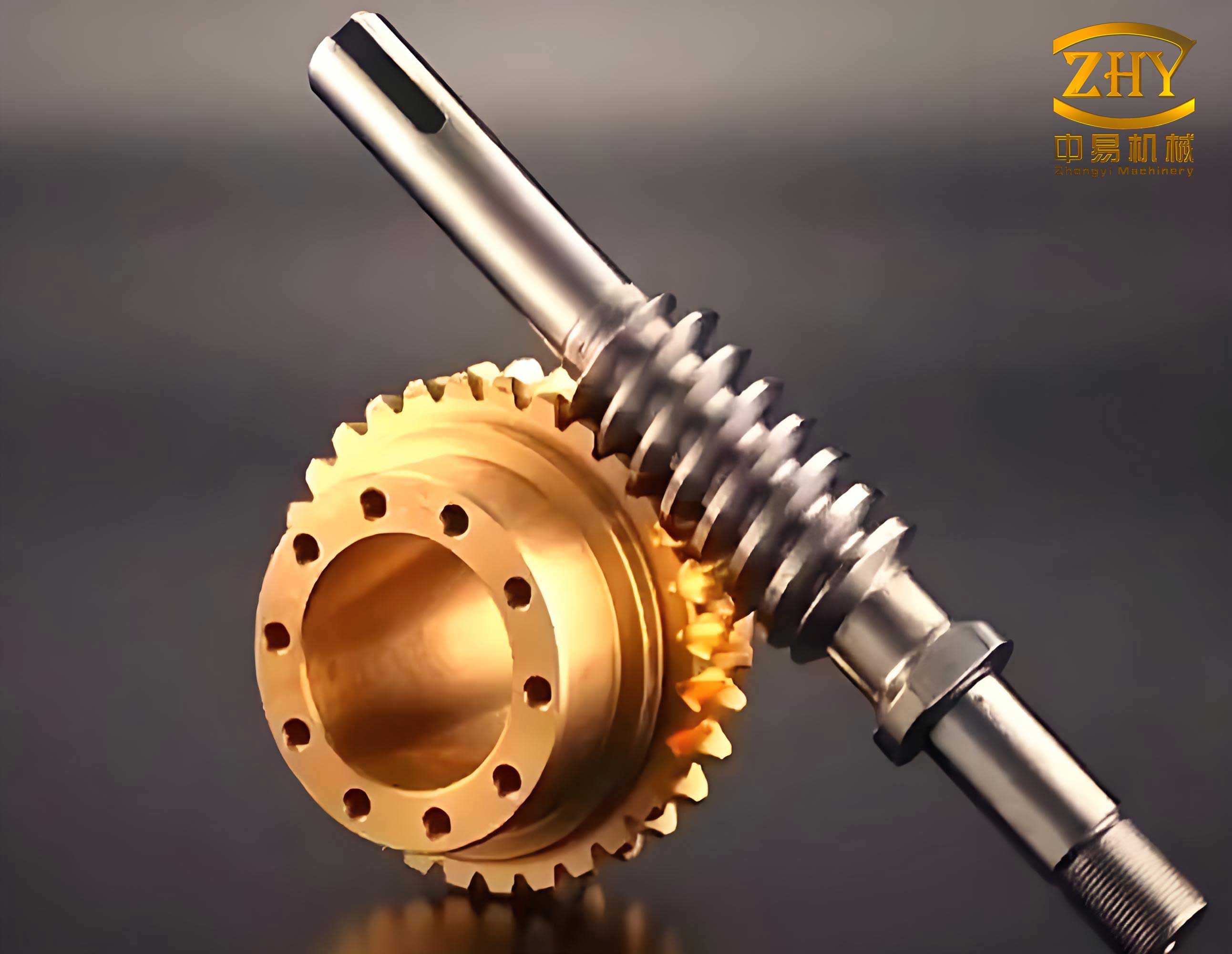
For the worm gear, a blank cylinder of diameter 336 mm and width 60 mm is created. The tool path equation in the worm gear coordinate system is implemented in Pro/E using a datum curve. The parameters are: \( r_1 = 40 \) mm, \( r_2 = m Z_2 / 2 = 160 \) mm, \( a = 200 \) mm, \( \omega_1 = 1 \) rad/s (scaled for parameter t), and \( \omega_2 = \omega_1 / i = 0.05 \) rad/s. The equation set is:
$$ \begin{cases} x = 40 \cdot \cos(t \cdot 360) + 200 \cdot \cos(0.05 \cdot t \cdot 360) – 160 \cdot \cos(0.05 \cdot t \cdot 360) \\ y = 40 \cdot \sin(t \cdot 360) + 200 \cdot \sin(0.05 \cdot t \cdot 360) – 160 \cdot \sin(0.05 \cdot t \cdot 360) \\ z = \text{Lead} \cdot t \end{cases} $$
with t from 0 to 1 and Lead as before. The tool profile is an involute sketch. The base radius \( r_b = r_2 \cos(\alpha) = 160 \cos(20°) = 150.351 \) mm. The involute is drawn using the equation curve in a sketch plane. The tooth space symmetry is set by calculating the angular offset. The pitch circle tooth thickness \( s = \pi m / 2 = 12.566 \) mm. On the base circle, the tooth thickness angle is computed, and the involute is mirrored accordingly. This closed profile is swept along the tool path with cut. The resulting tooth space is patterned 40 times around the axis. The final worm gear model exhibits true involute teeth in the mid-plane, ensuring correct meshing with the worm. To validate the screw gears assembly, both components are mated in Pro/E’s assembly module with appropriate constraints: the worm axis aligned to the worm gear axis with center distance 200 mm, and the threads engaged by rotational alignment. Interference analysis shows no collisions, confirming the accuracy of the models.
The advantages of this modeling approach for screw gears are multifold. First, it leverages standard CAD functionalities without requiring custom programming, making it accessible to engineers. Second, the models are parametrically driven; changes in design parameters like module, pressure angle, or number of teeth automatically update the geometry via Pro/E’s parametric associations. This is crucial for iterative design and optimization of screw gears. Third, the accurate digital prototypes facilitate downstream applications such as finite element analysis for stress evaluation, dynamic simulation for performance prediction, and manufacturing planning for CNC toolpaths. Moreover, the method is not limited to Archimedes screw gears; it can be adapted to other worm profiles (e.g., involute or convolute) by modifying the tool geometry and trajectory equations. For instance, for involute helicoid worms, the tool path would involve a different mathematical formulation, but the Pro/E workflow remains similar. This versatility underscores the robustness of simulation-based modeling for screw gears.
To further enhance the utility, we can integrate these modeling steps into Pro/E’s Family Table or User-Defined Features (UDFs) for standard screw gear libraries. Designers can then select from a catalog of screw gears, input key parameters, and instantly generate 3D models. Additionally, the mathematical models can be extended to account for manufacturing tolerances, misalignments, and lubrication gaps, leading to more realistic simulations. The table below summarizes the key equations used in the modeling process for Archimedes screw gears, providing a quick reference for implementation.
| Component | Equation Type | LaTeX Formula | Purpose |
|---|---|---|---|
| Worm Tool Path | Helical Trajectory | $$ \begin{cases} x = r \cos(\omega t) \\ y = r \sin(\omega t) \\ z = v t \end{cases} $$ | Define sweep path for worm tooth cut |
| Worm Gear Tool Path | Complex Helix | $$ \begin{cases} x_2 = r_1 \cos(\omega_1 t) + a \cos(\omega_2 t) – r_2 \cos(\omega_2 t) \\ y_2 = r_1 \sin(\omega_1 t) + a \sin(\omega_2 t) – r_2 \sin(\omega_2 t) \\ z_2 = v t \end{cases} $$ | Define sweep path for worm gear tooth cut |
| Involute Profile | Curve Equation | $$ \begin{cases} x = r_b (\cos(\theta) + \theta \sin(\theta)) \\ y = r_b (\sin(\theta) – \theta \cos(\theta)) \end{cases} $$ | Define tooth shape for worm gear |
| Tooth Thickness | Geometric Relation | $$ s_k = s \frac{r_k}{r} – 2 r_k (\text{inv}(\alpha_k) – \text{inv}(\alpha)) $$ | Calculate tooth width at any radius |
In conclusion, this paper demonstrates a practical method for precise three-dimensional modeling of Archimedes screw gears in Pro/E by simulating their machining processes. The approach involves deriving mathematical models for tool trajectories and tooth profiles, then implementing them using Pro/E’s built-in curve and sweep features. The resulting digital models are accurate and suitable for advanced engineering analyses. The methodology is efficient, requiring no secondary development, and can be extended to other types of screw gears and gear systems. By adopting this simulation-based strategy, designers can significantly streamline the design and validation of screw gears, reducing time and cost while improving product quality. Future work could focus on automating the parameter input via Pro/E’s programming interface, integrating with optimization algorithms, and expanding to multi-axis machining simulations for advanced screw gear forms.