
The study of gear geometry, particularly for specialized types like screw gears, remains a critical area for advancing power transmission efficiency and durability. Among these, the globoidal worm drive, a specific and historically significant form of worm gear, presents unique challenges and opportunities. This drive is characterized by a worm shaped to partially envelop the worm wheel, offering high single-stage reduction ratios and potential for compact design. However, its traditional form suffers from significant limitations that hinder optimal performance. This work delves into a systematic mathematical and analytical exploration of a high-order modification methodology aimed at overcoming these inherent drawbacks. The focus is on the straight-sided (or Hindley) type, where the worm thread profile in its axial section is a straight line, simplifying tool geometry but introducing specific meshing constraints.
The primary limitation of the conventional, or “primitive,” straight-sided globoidal worm drive is the presence of a so-called “constant contact line” on the worm wheel tooth surface. This phenomenon results in an extremely limited conjugate contact area, concentrating stress and leading to premature wear and failure. To address this, modification techniques have been developed. These can be broadly classified into empirical “natural modification,” based on measured wear patterns, and theoretical “rational modification,” based on deliberate alterations of the gear generation kinematics. This paper focuses on formalizing and generalizing a high-order polynomial approach derived from the principles of natural modification, establishing a universal mathematical framework for its analysis. We will develop the complete geometric model, derive essential meshing parameters, and critically evaluate the performance outcomes through numerical simulation, connecting the analysis to broader considerations in the design of robust screw gears.
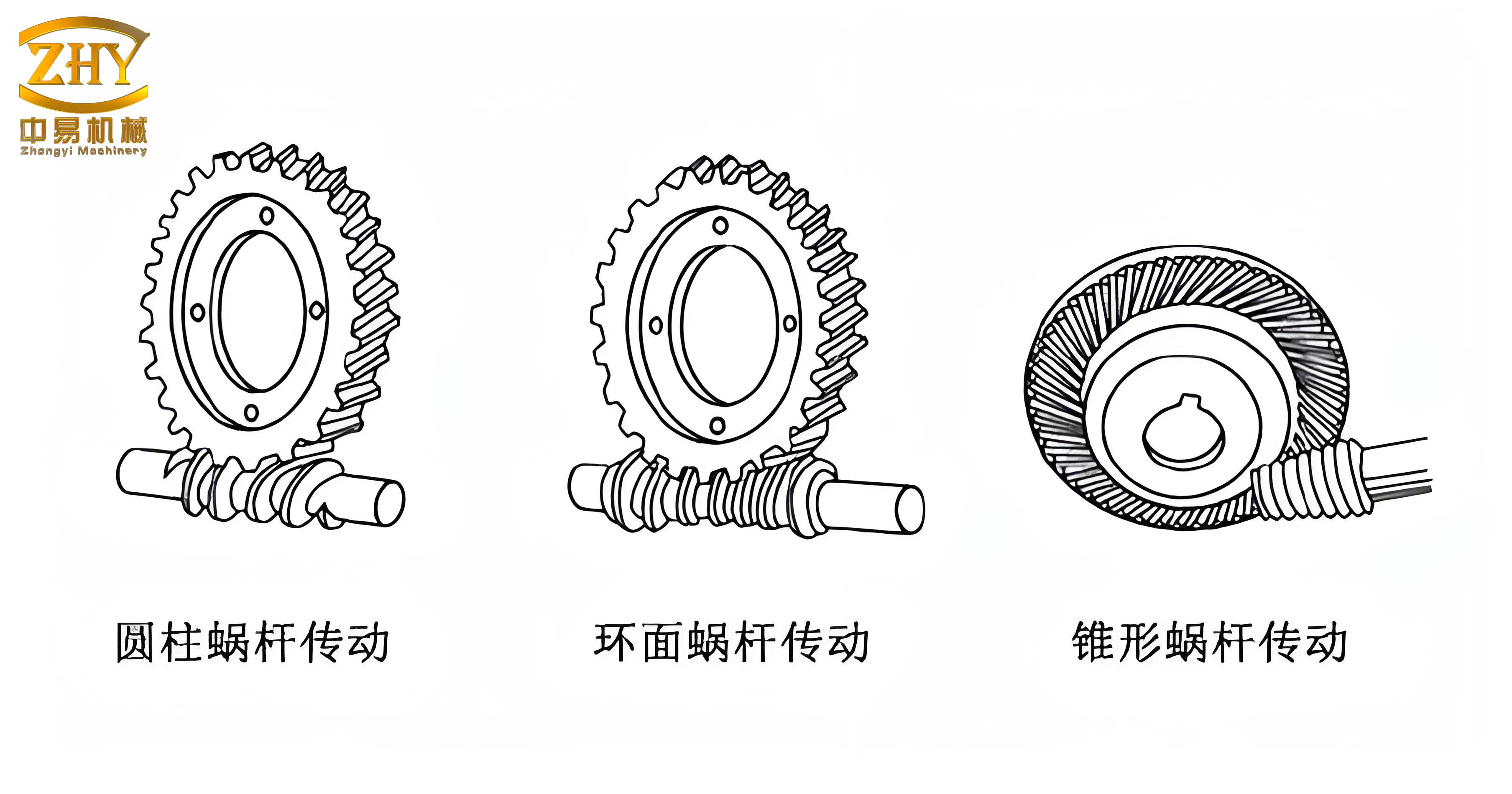
The mathematical foundation begins with the coordinate systems describing the worm generation process. The worm surface \(\Sigma_1\) is generated by a straight-edged cutting tool. Let us define a moving coordinate system \(\sigma_d = [O_d; \vec{i_d}, \vec{j_d}, \vec{k_d}]\) attached to the cutting tool. The equation of the straight cutting edge in \(\sigma_d\) is given by:
$$\vec{r_d}^{(d)} = -u \vec{i_d} + r_b \vec{j_d}$$
where \(u\) is the tool profile parameter and \(r_b\) is the base circle radius of the worm. During generation, the tool rotates with an angle \(\varphi_d\) relative to the worm blank, which itself rotates with an angle \(\varphi\). The relationship between these angles is key to modification and is given by the process transmission ratio \(i_{1d} = d\varphi / d\varphi_d\). For the primitive design, \(i_{1d} = i_{12}\), the nominal gear ratio. For the modified drive, \(i_{1d}\) becomes a function of \(\varphi\).
Using rotation matrices \(\mathbf{R}[\vec{k}, \theta]\), the family of cutting edge positions in the fixed tool frame \(\sigma_{od}\) and subsequently the generated worm surface in the worm coordinate system \(\sigma_1 = [O_1; \vec{i_1}, \vec{j_1}, \vec{k_1}]\) can be derived. The resulting worm surface equation is:
$$\vec{r_1}^{(1)}(u, \varphi) = \mathbf{R}[\vec{k_1}, -\varphi] \left( a \vec{i_{o1}} + \mathbf{R}[\vec{i_{o1}}, \pi/2] \vec{r_d}^{(od)} \right)$$
where \(a\) is the nominal center distance and \(\vec{r_d}^{(od)} = \mathbf{R}[\vec{k_{od}}, \varphi_d] \vec{r_d}^{(d)}\). This surface can be recognized as a ruled surface: \(\vec{r_1}^{(1)} = \vec{\rho}(\varphi) + u \vec{t}(\varphi)\). To prove it is non-developable, we compute the scalar triple product:
$$[\vec{\rho}^{\,’}(\varphi), \vec{t}(\varphi), \vec{t}^{\,’}(\varphi)] = \frac{1}{i_{1d}}(a – r_b \sin \varphi_d) \neq 0$$
Since this product is non-zero, the ruled surface is confirmed to be non-developable, aligning with the known geometrical properties of this worm type and impacting its manufacturability via grinding.
The fundamental quantities of the worm surface are essential for meshing analysis. The first derivatives yield the first fundamental form coefficients \(E, F, G\):
$$E = \vec{r_{1u}} \cdot \vec{r_{1u}} = 1, \quad F = \vec{r_{1u}} \cdot \vec{r_{1\varphi}} = \frac{r_b}{i_{1d}}, \quad G = \vec{r_{1\varphi}} \cdot \vec{r_{1\varphi}} = \frac{(x_{od}+a)^2 + u^2 + r_b^2}{i_{1d}^2}$$
where \(x_{od} = -u \cos \varphi_d – r_b \sin \varphi_d\). The surface unit normal vector is:
$$\vec{n_1}^{(1)} = \frac{\vec{r_{1u}} \times \vec{r_{1\varphi}}}{\sqrt{EG-F^2}} = \frac{1}{D} \mathbf{R}[\vec{k_1}, -\varphi] \mathbf{R}[\vec{i_{o1}}, \pi/2] \mathbf{R}[\vec{k_{od}}, \varphi_d] \left[ (a+x_{od})\vec{j_d} + \frac{u}{i_{1d}}\vec{k_d} \right]$$
with \(D = \sqrt{(u/i_{1d})^2 + (a+x_{od})^2}\). The second fundamental form coefficients \(L, M, N\) are calculated using the second derivatives and the unit normal:
$$L=0, \quad M = \frac{r_b \sin \varphi_d – a}{i_{1d} D}, \quad N = \frac{a+x_{od}}{D} \left( (a+x_{od})\sin \varphi_d – u \frac{d^2\varphi_d}{d\varphi^2} – \frac{r_b}{i_{1d}^2} \right) – \frac{2u y_{od}}{i_{1d}^2 D}$$
From these, the normal curvature \(k_\xi\) and geodesic torsion \(\tau_g\) along the generating line direction (\(\vec{\alpha_\xi} = \vec{t}(\varphi)\)) and the mean curvature \(H\) are:
$$k_\xi = \frac{L}{E} = 0, \quad \tau_g = \frac{EM – FL}{D^2} = \frac{M}{D}, \quad H = \frac{EN – 2FM + GL}{2D^2} = \frac{N – 2FM}{2D^2}$$
The meshing condition between the worm and the worm wheel is governed by the equation \(\Phi(u, \varphi, \varphi_1)=0\), where \(\varphi_1\) is the wheel’s rotation angle. The relative velocity \(\vec{V}_{12}\) and the unit normal \(\vec{n}^*\) are computed in a fixed frame. The meshing function is:
$$\Phi(u, \varphi, \varphi_1) = \vec{n}^* \cdot \vec{V}_{12} = \frac{1}{i_{12}D} \left[ A \sin(\varphi_1-\varphi) + B \cos(\varphi_1-\varphi) + C \right] = 0$$
where the coefficients are:
$$A = \frac{u y_{od}}{i_{1d}}, \quad B = (x_{od}+a)(u – a \cos \varphi_d), \quad C = (x_{od}+a)\left( a \cos \varphi_d – \frac{i_{12}}{i_{1d}}u \right)$$
Solving \(\Phi=0\) yields two solutions for \(\varphi_1\), corresponding to two conjugate zones \(\Sigma_A\) and \(\Sigma_B\) on the worm wheel tooth surface. The worm wheel surface \(\Sigma_2\) in its own frame \(\sigma_2\) is then obtained via coordinate transformation of \(\vec{r_1}^{(1)}\) under the condition \(\Phi=0\):
$$\vec{r_2}^{(2)} = \mathbf{R}[\vec{k_2}, -\varphi_1/i_{12}] \left\{ \mathbf{R}[\vec{i_{o2}}, -\pi/2] \vec{r_1}^{\,(o1)} – a \vec{i_{o2}} \right\}$$
A critical aspect of meshing analysis is identifying the limit of contact where undercutting or severe curvature interference may occur. This is found via the curvature interference boundary function \(\Psi\):
$$\Psi = N_\xi (\vec{V}_{12}\cdot\vec{\alpha_\xi}) + N_\eta (\vec{V}_{12}\cdot\vec{\alpha_\eta}) + \Phi_{\varphi_1}$$
where \(N_\xi\) and \(N_\eta\) are components of the normal vector to the instantaneous contact line, and \(\Phi_{\varphi_1} = \partial \Phi / \partial \varphi_1\). The induced normal curvature \(k_N^{(12)}\) and the sliding angle \(\theta_{vt}\), which is indicative of lubricant entrainment conditions, are:
$$k_N^{(12)} = \frac{N_\xi^2 + N_\eta^2}{\Psi}, \quad \theta_{vt} = \arcsin\left( \frac{|\Psi – \Phi_{\varphi_1}|}{|\vec{V}_{12}| \sqrt{N_\xi^2+N_\eta^2}} \right)$$
The core of the proposed modification lies in defining the process transmission ratio \(i_{1d}(\varphi)\) based on a high-order polynomial correction curve. Empirical wear data is first normalized. Let \(\varphi_x = \alpha – \varphi/i_{12}\) be the nominal tool angle, where \(\alpha\) is the pressure angle. Define a normalized angle parameter \(x = \varphi_x / \varphi_w\), where \(\varphi_w\) is the worm wrap angle. The modification amount \(\Delta\) is normalized by the entry-end modification \(\Delta_f\): \(I_i = \Delta^{(i)}/\Delta_f\). Using least-squares fitting on normalized data, a universal high-order modification curve is established:
$$I_n(x) = \sum_{k=0}^{n} c_k x^k, \quad \text{and thus} \quad \Delta(x) = \Delta_f I_n(x)$$
The relationship between the modification and the tool’s auxiliary rotation \(\Delta \varphi_d\) is \(\Delta \varphi_d = \Delta / r_2\), where \(r_2\) is the worm wheel pitch radius. Consequently, the actual tool rotation angle becomes \(\varphi_d = \varphi/i_{12} – \Delta_f I_n(x)/r_2\). The variable process transmission ratio is then:
$$i_{1d}(x) = \frac{1}{d\varphi_d/d\varphi} = \frac{i_{12}}{1 + \frac{\Delta_f}{r_2 \varphi_w} I_n'(x)} \quad \text{where} \quad I_n'(x) = \sum_{k=1}^{n} k c_k x^{k-1}$$
This equation directly links the high-order polynomial correction to the generation kinematics, making \(i_{1d}\) a function of the worm rotation angle \(\varphi\). The coefficients for polynomials of degrees 3 to 7, derived from fitting, are shown below:
| Coefficient | Cubic (n=3) | Quartic (n=4) | Quintic (n=5) | 6th Order (n=6) | 7th Order (n=7) |
|---|---|---|---|---|---|
| \(c_0\) | 9.9857E-02 | 1.0202E-01 | 1.0202E-01 | 9.6396E-02 | 9.640E-02 |
| \(c_1\) | 5.0056E-01 | 5.0056E-01 | 5.2125E-01 | 5.2125E-01 | 5.1184E-01 |
| \(c_2\) | 4.2790E-01 | 4.0739E-01 | 4.0739E-01 | 5.2004E-01 | 5.2004E-01 |
| \(c_3\) | -4.5089E-02 | -4.5089E-02 | -1.3687E-01 | -1.3687E-01 | -5.5751E-02 |
| \(c_4\) | – | -2.2659E-02 | 2.2659E-02 | -2.9935E-01 | -2.9935E-01 |
| \(c_5\) | – | – | 7.8395E-02 | 7.8395E-02 | -9.2200E-02 |
| \(c_6\) | – | – | – | 2.2474E-01 | 2.2474E-01 |
| \(c_7\) | – | – | – | – | 1.0084E-01 |
For a numerical case study, consider a worm drive with the following parameters: center distance \(a = 280\) mm, nominal transmission ratio \(i_{12}=25\), worm threads \(Z_1=2\). Key derived parameters are calculated using standard design formulas for screw gears:
| Parameter | Symbol | Value / Formula |
|---|---|---|
| Worm Pitch Diameter | \(d_1\) | |
| Wheel Pitch Diameter | \(d_2\) | \(2a – d_1 = 466\) mm |
| Wheel Face Width | \(b_2\) | \(0.25a = 70\) mm |
| Base Circle Diameter | \(d_b\) | \(\approx 0.625a = 175\) mm |
| Pressure Angle | \(\alpha\) | \(\arcsin(d_b/d_2) = 22.06^\circ\) |
| Wheel Teeth Number | \(Z_2\) | \(i_{12}Z_1 = 50\) |
| Wrap Angle | \(\varphi_w\) | \(\pi (Z_2/10 – 0.5)/Z_2 = 16.38^\circ\) |
| Entry-end Modification | \(\Delta_f\) | \(a(0.0003+0.000034i_{12}) = 0.3239\) mm |
Analysis of the primitive drive (\(i_{1d} \equiv i_{12}\)) confirms its critical flaw. The conjugate zone \(\Sigma_A\) on the worm wheel collapses into a single “constant contact line.” The secondary zone \(\Sigma_B\) exists but is limited. While the induced normal curvature \(k_N^{(12)}\) in \(\Sigma_B\) is low and the sliding angle \(\theta_{vt}\) is favorable (often above \(60^\circ\)), the infinitesimal contact area renders the design impractical for sustained load.
Applying the high-order modification transforms the meshing characteristics. For the cubic (\(n=3\)) and quintic (\(n=5\)) modifications, the conjugate zone \(\Sigma_A\) is restored as a true area, eliminating the constant contact line. The zone \(\Sigma_B\) expands to utilize the full length of the worm thread. However, a curvature interference line (\(GH\), where \(\Psi=0\)) appears within \(\Sigma_A\), posing a risk of undercutting if it intersects the active tooth profile. The modification successfully creates a double-line contact region near the entry. The table below summarizes the meshing quality indicators at characteristic points for different modification schemes, showing the impact on induced curvature and sliding angle.
| Mod Type & Point | Zone | \(k_N^{(12)}\) (mm\(^{-1}\)) | \(\theta_{vt}\) (deg) | Notes |
|---|---|---|---|---|
| Primitive (Point on 1′) | \(\Sigma_B\) | 0.0065 | 48.0 | Low stress, good slip. |
| Cubic (Point on 1) | \(\Sigma_A\) | 0.1170 | 83.5 | Higher curvature but excellent slip angle. |
| Cubic (Point on 5′) | \(\Sigma_B\) | 0.0155 | 83.2 | Good performance in expanded zone. |
| Quintic (Point on 1) | \(\Sigma_A\) | 0.0388 | 83.5 | Curvature reduced vs. cubic; excellent slip. |
| 7th Order (Point on 1) | \(\Sigma_A\) | 0.0144 | 83.4 | Further reduced curvature, favorable conditions. |
Increasing the polynomial order to \(n=7\) offers further refinement. The conjugate zone \(\Sigma_A\) enlarges significantly. Notably, part of the exit boundary from zone \(\Sigma_B\) now lies beyond the curvature interference line \(GH\) of zone \(\Sigma_A\). This implies that the segment of the interference line near the wheel root can be theoretically removed from the active profile, mitigating the undercutting risk. However, the instantaneous contact lines within \(\Sigma_A\) become densely packed near this boundary, indicating a region of higher contact frequency and potential susceptibility to pitting. As the data in the table shows, the 7th-order modification achieves a very low induced normal curvature in \(\Sigma_A\) while maintaining superb sliding angles, suggesting improved contact stress and lubrication conditions compared to lower-order modifications.
In conclusion, this study has established a rigorous mathematical framework for the high-order modification of straight-sided globoidal worm drives, a specialized and demanding class of screw gears. The key achievement is the derivation of a universal, normalized high-order polynomial correction curve and its explicit integration into the generation kinematics via a variable process transmission ratio \(i_{1d}(\varphi)\). This approach fundamentally addresses the crippling limitation of the constant contact line, transforming it into a sizeable conjugate area and enabling full utilization of the worm thread length. The mathematical proof of the worm surface being a non-developable ruled surface is consistent with its known geometric properties.
The numerical analysis confirms the efficacy of high-order modification. It significantly expands the contact area, introduces a beneficial double-line contact region, and maintains favorable local meshing conditions (low induced curvature and high sliding angles) conducive to load capacity and fluid film formation. However, the analysis also reveals a persistent challenge: the emergence of a curvature interference boundary within the primary contact zone. While increasing the modification order can reduce the severity and extent of this boundary, it is difficult to eliminate entirely through this method alone. This interference poses a potential for localized undercutting or excessively high contact stress. Therefore, while high-order natural modification represents a substantial improvement over the primitive design, its practical implementation is complicated by the need for a variable process transmission ratio during manufacturing and the inherent presence of a sensitive curvature boundary. For optimal performance in demanding applications, a synthesis of this approach with other rational modification parameters (e.g., adjusted center distance or tool tilt) may be necessary to fully control the contact pattern and eliminate detrimental interference, pushing the performance boundaries of this type of enveloping screw gear.