
In the field of mechanical transmission design, screw gears, encompassing worm and worm wheel systems, are pivotal components for achieving high reduction ratios and compact design in a single stage. Their unique non-parallel, non-intersecting shaft configuration and sliding-dominant contact necessitate meticulous design and analysis to ensure efficiency, durability, and accurate kinematic performance. This article details a proven methodology for the design and dynamic simulation of screw gears, leveraging the synergistic strengths of parametric CAD and multi-body dynamics (MBD) software. The core workflow involves constructing a precise three-dimensional model, seamlessly transferring it to a dynamics environment, defining the physical interactions, and performing motion simulation to validate theoretical calculations. This integrated approach significantly enhances design confidence and reduces reliance on physical prototyping.
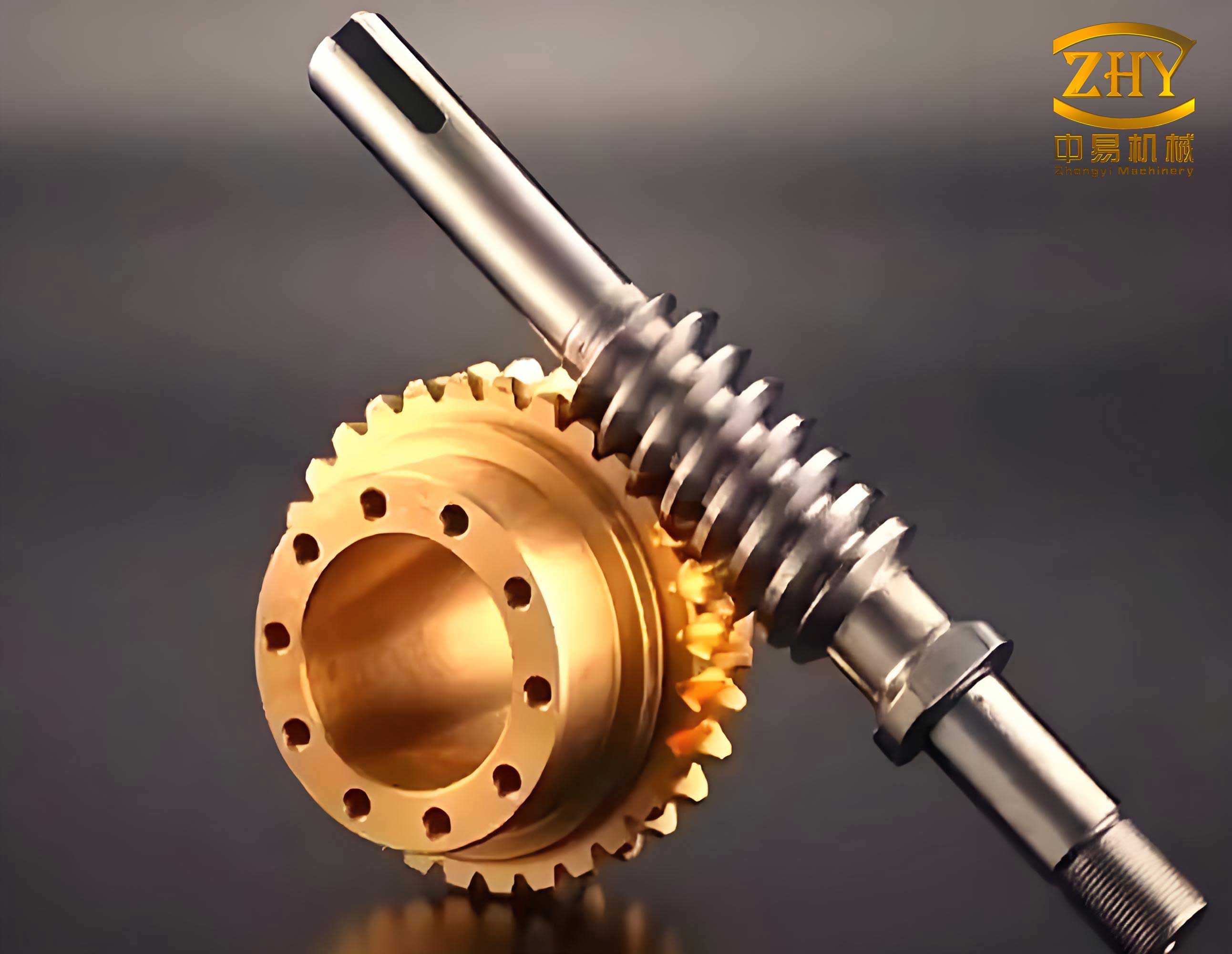
The foundation of any accurate simulation is a geometrically precise digital model. For screw gears, this begins with parametric modeling using advanced CAD software. The key parameters for a standard cylindrical screw gear set include the axial module (m), the number of threads on the worm (often considered as its “齿数” Z1, typically 1, 2, or 4), the number of teeth on the worm wheel (Z2), the diameter quotient (q), which defines the worm’s pitch diameter relative to the module, and the pressure angle (α). For a given design with m=2, Z2=28, q=7, and α=20°, the primary dimensions are calculated as follows:
The pitch diameter of the worm, d1:
$$ d1 = m \times q = 2 \times 7 = 14 \text{ mm} $$
The pitch diameter of the worm wheel, d2:
$$ d2 = m \times Z2 = 2 \times 28 = 56 \text{ mm} $$
The lead angle of the worm on the pitch cylinder, γ, is crucial for determining the transmission ratio and efficiency:
$$ \tan(\gamma) = \frac{m \times Z1}{d1} = \frac{Z1}{q} $$
For a single-start worm (Z1=1), this gives:
$$ \gamma = \arctan(1/7) \approx 8.13^\circ $$
Using these parameters, the three-dimensional solid models of the worm and the worm wheel are generated. The worm profile is created as a helical sweep with a trapezoidal tooth section, while the worm wheel is typically modeled using specialized gear creation tools or by performing a Boolean subtraction of the properly positioned worm from a gear blank, ensuring conjugate tooth forms. The components are then virtually assembled with appropriate constraints to align their axes correctly and establish the nominal center distance, a = (d1 + d2)/2 = 35 mm.
A critical and often challenging step is the accurate transfer of the assembled CAD model to the MBD environment. Not all file formats preserve geometric and assembly data flawlessly. Experience shows that the Parasolid format offers superior robustness for this data exchange. Since some CAD systems may not export directly to this format, an intermediary step using a neutral format like STEP, followed by conversion in a compatible tool, is recommended. This process helps maintain model integrity, ensuring that the MBD software correctly recognizes individual components as separate rigid bodies, a prerequisite for defining joints and contacts.
Upon successful import, the model in the MBD environment consists of the worm, the worm wheel, and the ground (frame). The first task is to define the kinematic joints that constrain their motion. Two revolute joints are created:
- Joint_Worm: Connects the worm to the ground, allowing only rotation about its own axis.
- Joint_Wheel: Connects the worm wheel to the ground, allowing only rotation about its own axis.
The precise location and orientation of these joints are critical and should align with the theoretical axes of rotation defined during the CAD modeling phase.
The defining interaction for screw gears is established not through a standard contact force but via a gear pair constraint. This kinematic constraint directly enforces the velocity relationship between the two connected revolute joints at a specific point. The most critical and nuanced part of this setup is the correct placement and orientation of the common velocity marker (the啮合点). This marker must lie on the line connecting the two joint centers, and its orientation defines the direction of the velocity transfer.
Let the position of the worm’s joint marker be \( \vec{P}_1 \) and the worm wheel’s joint marker be \( \vec{P}_2 \). The line connecting them is \( \vec{L} = \vec{P}_2 – \vec{P}_1 \). The gear pair marker \( \vec{P}_3 \) must lie on this line. Its exact location can be derived from the transmission ratio, i. For screw gears, the theoretical velocity ratio is:
$$ i = \frac{\omega_1}{\omega_2} = \frac{Z2}{Z1} $$
Where \( \omega_1 \) and \( \omega_2 \) are the angular velocities of the worm and worm wheel, respectively. The kinematic relationship at the pitch point is:
$$ \omega_1 \cdot r1′ \cdot \tan(\gamma’) = \omega_2 \cdot r2′ $$
Here, \( r1′ \) and \( r2′ \) are the operating pitch radii, and \( \gamma’ \) is the operating lead angle. For properly designed screw gears with standard center distance, these are approximately equal to the nominal values. Therefore, the position of the common marker \( \vec{P}_3 \) along the line \( \vec{L} \) can be approximated based on the ratio of angular velocities. More precisely, its coordinates are often found by selecting the apparent point of contact or calculated via the geometry of the pitch surfaces.
The orientation of this marker is paramount. Its z-axis must be aligned with the common normal to the tooth surfaces at the point of contact, which, for screw gears, is related to the lead and pressure angles. A typical orientation, expressed in body-fixed Euler angles, might be (270, 90-γ, 180) degrees to align the local coordinate system correctly with the driving direction. An incorrect orientation will produce erroneous velocity relations. The table below summarizes the key parameters for establishing the screw gear pair:
| Parameter | Symbol | Value / Description |
|---|---|---|
| Worm Revolute Joint | Joint_Worm | Connects Worm to Ground |
| Wheel Revolute Joint | Joint_Wheel | Connects Worm Wheel to Ground |
| Transmission Ratio | i | Z2 / Z1 = 28 (for Z1=1) |
| Common Velocity Marker Location | P3 | Lies on line between joint centers |
| Common Velocity Marker Orientation | (ψ, θ, φ) | e.g., (270, 81.87, 180) for γ=8.13° |
Finally, a motion driver is applied to the worm’s revolute joint to prescribe its rotation. For instance, a rotational velocity of 360 deg/s (or 2π rad/s) is a common input for simulation. The simulation is then run for a specified time, and the resulting motion of the worm wheel is measured.
The primary output of the dynamic simulation is the kinematic response. By measuring the angular velocity of the worm wheel (\( \omega_{2, sim} \)), the simulated transmission ratio can be calculated and compared to the theoretical value:
$$ i_{sim} = \frac{\omega_{1, input}}{\omega_{2, sim}} $$
For the example with a single-start worm (Z1=1, Z2=28), the theoretical ratio is 28:1. If the input worm speed is 360 deg/s, the expected output speed for the worm wheel is:
$$ \omega_{2, expected} = \frac{\omega_{1, input}}{i} = \frac{360}{28} \approx 12.857 \text{ deg/s} $$
A well-configured simulation will yield a result extremely close to this value. The direction of rotation should also correspond to the hand of the worm’s helix. The results validate not just the ratio but the correctness of the entire setup—the joint locations, the gear pair definition, and the marker orientation. The table below contrasts the theoretical and simulated performance for a typical case:
| Performance Metric | Theoretical Value | Simulated Value | Notes |
|---|---|---|---|
| Input Speed (Worm) | 360 deg/s | 360 deg/s (Prescribed) | Driver condition |
| Output Speed (Wheel) | -12.857 deg/s | -12.86 deg/s | Negative indicates opposite direction |
| Transmission Ratio (i) | 28.0 | ≈ 28.0 | i = |ω_worm / ω_wheel| |
| Kinematic Consistency | N/A | High | Smooth, constant velocity output |
This integrated approach for screw gear simulation offers substantial advantages over traditional, disjointed design methods. The parametric CAD model ensures geometric accuracy and easy design modification. The use of a robust Parasolid data interface maintains model fidelity during transfer. The MBD environment, with its precise gear pair constraint, allows for the efficient and accurate analysis of complex spatial kinematics without the computational expense of resolving transient contact forces for basic motion validation. This methodology enhances design insight, accelerates the iterative design process, and reduces the costs and risks associated with physical prototyping. It provides a virtual proving ground where the motion characteristics of screw gears can be thoroughly evaluated and optimized before manufacturing.
Further analysis can be extended by replacing the kinematic gear pair with a force-based contact definition, which would allow for the investigation of dynamic loads, contact pressures, and efficiency losses due to friction—critical aspects for the detailed mechanical design of durable screw gear systems. However, for fundamental kinematic validation and motion path verification, the described process utilizing a correctly defined gear pair is both efficient and sufficiently accurate.