
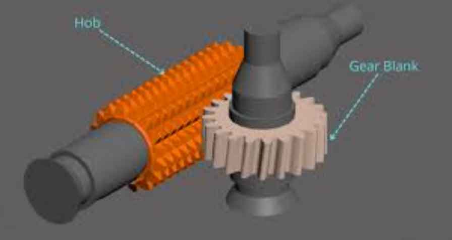
In the realm of modern gear manufacturing, high-speed dry gear hobbing has emerged as a pivotal green machining technology. This process eliminates the need for cutting fluids, thereby reducing environmental impact and operational costs, while simultaneously achieving significant reductions in machining cycle times. However, the quest for optimal performance in high-speed dry gear hobbing is often complicated by the multi-variable, multi-objective nature of the process. Parameters such as feed rate, hob rotational speed, hob diameter, and number of hob starts interact in complex ways, influencing conflicting objectives like minimizing machining time and minimizing machining cost. A common challenge is the presence of too many variables to optimize simultaneously and the inherent conflicts between parameter selections for different goals. To address this, a systematic approach for identifying the most influential parameters is crucial before embarking on optimization. This article presents a methodology that employs global sensitivity analysis to screen and prioritize process parameters, followed by multi-objective optimization, providing a robust theoretical framework for parameter selection in high-speed dry gear hobbing.
Mathematical Modeling of Key Performance Indicators
The effectiveness of any optimization strategy hinges on accurate mathematical models that describe the relationship between input process parameters and output performance measures. For high-speed dry gear hobbing, two primary objectives are often considered: total machining time per gear and total machining cost per gear.
1. Machining Time Model
The total machining time (T) for a single gear is not merely the cutting time. It is an aggregate of the setup time, the actual cutting time, and the time attributed to tool changes over the tool’s life. The formula is expressed as:
$$ T = t_p + t_m + t_c \left( \frac{t_m}{t_l} \right) $$
Where:
\( t_p \) = Preparation/setup time (min).
\( t_m \) = Actual hobbing machining time (min/piece).
\( t_c \) = Tool change time (min/change).
\( t_l \) = Tool life (min).
The core machining time \( t_m \) is calculated based on the total axial travel of the hob and the feed dynamics:
$$ t_m = \frac{L_1 + B + L_2}{f_a \cdot n_0} \times \frac{z_2}{k} $$
Where:
\( L_1 \) = Hob approach distance (mm).
\( B \) = Gear width (mm).
\( L_2 \) = Hob overtravel distance (mm).
\( f_a \) = Axial feed rate (mm/rev of workpiece).
\( n_0 \) = Hob rotational speed (rpm).
\( z_2 \) = Number of teeth on the gear.
\( k \) = Number of hob starts.
Tool life \( t_l \) in gear hobbing is typically modeled using a modified Taylor’s tool life equation, incorporating key process parameters:
$$ t_l = \left( \frac{C_v}{v \cdot f_a^{y_v} \cdot m^{x_v} \cdot k_v} \right)^{\frac{1}{m_v}} $$
Where:
\( v \) = Cutting speed (m/min), related to hob speed by \( v = \frac{\pi n_0 d_{a0}}{1000} \).
\( d_{a0} \) = Hob diameter (mm).
\( m \) = Gear module.
\( C_v, m_v, x_v, y_v \) = Empirical constants dependent on the tool-workpiece material pair.
\( k_v \) = A product of various correction factors for material, hob geometry, and cutting conditions.
Since setup time \( t_p \) is generally a fixed constant for a given batch and does not participate in process parameter optimization, the final model for machining time per gear simplifies to:
$$ T = \frac{(L_1 + B + L_2) \cdot z_2}{f_a \cdot n_0 \cdot k} + t_c \left[ \frac{(L_1 + B + L_2) \cdot z_2}{f_a \cdot n_0 \cdot k} \times \left( \frac{1000 \cdot C_v}{\pi \cdot f_a^{y_v} \cdot d_{a0} \cdot n_0 \cdot m^{x_v} \cdot k_v} \right)^{-\frac{1}{m_v}} \right] $$
2. Machining Cost Model
Similarly, the total machining cost per gear (C) encompasses direct and indirect costs:
$$ C = C_m + M \cdot t_p + M \cdot t_m + (M \cdot t_c + C_t)\left( \frac{t_m}{t_l} \right) $$
Where:
\( C_m \) = Raw material cost per piece (constant).
\( M \) = Machine and labor overhead rate (cost per unit time).
\( C_t \) = Cost per cutting edge or per hob regrind.
Omitting the constant raw material cost \( C_m \) and the fixed setup cost component \( M \cdot t_p \), the optimizable cost model becomes:
$$ C = M \cdot \frac{(L_1 + B + L_2) \cdot z_2}{f_a \cdot n_0 \cdot k} + (M \cdot t_c + C_t) \left[ \frac{(L_1 + B + L_2) \cdot z_2}{f_a \cdot n_0 \cdot k} \times \left( \frac{1000 \cdot C_v}{\pi \cdot f_a^{y_v} \cdot d_{a0} \cdot n_0 \cdot m^{x_v} \cdot k_v} \right)^{-\frac{1}{m_v}} \right] $$
These two equations, (6) and (8), form the foundational objective functions for our analysis. They are complex, non-linear functions of multiple input parameters.
Sobol’s Method for Global Sensitivity Analysis
When dealing with multi-parameter, non-linear models, local sensitivity analyses (e.g., derivative-based methods) are insufficient as they evaluate sensitivity at a single point in the parameter space. A global sensitivity analysis (GSA) is required to apportion the output uncertainty to the uncertainty in the input parameters over their entire feasible ranges. Sobol’s method, a variance-based GSA technique, is particularly powerful for this purpose. It quantifies how much of the total variance in the output (e.g., machining time T) is caused by the variance in each input parameter alone, and by the interactions between them.
The core idea is to decompose the model function \( f(\mathbf{x}) \), where \( \mathbf{x} = (x_1, x_2, …, x_k) \) are the k input parameters, into summands of increasing dimensionality:
$$ f(\mathbf{x}) = f_0 + \sum_{i=1}^{k} f_i(x_i) + \sum_{1 \le i < j \le k} f_{ij}(x_i, x_j) + … + f_{1,2,…,k}(x_1, x_2, …, x_k) $$
Here, \( f_0 \) is the mean value of the function. \( f_i(x_i) \) describes the effect of varying parameter \( x_i \) alone (the first-order effect). \( f_{ij}(x_i, x_j) \) describes the synergistic effect of varying \( x_i \) and \( x_j \) together that is not explained by their individual effects (the second-order interaction effect). Higher-order terms capture more complex interactions.
Assuming the inputs are independent, the total variance \( D \) of the output is:
$$ D = \int_{\Omega^k} f^2(\mathbf{x}) d\mathbf{x} – f_0^2 $$
This total variance can be decomposed similarly:
$$ D = \sum_{i=1}^{k} D_i + \sum_{1 \le i < j \le k} D_{ij} + … + D_{1,2,…,k} $$
Where \( D_i \) is the partial variance attributable solely to \( x_i \), \( D_{ij} \) is the partial variance due to the interaction between \( x_i \) and \( x_j \), and so on.
The sensitivity indices are then defined as ratios of these partial variances to the total variance:
- First-Order Sensitivity Index (\( S_i \)): \( S_i = \frac{D_i}{D} \). This measures the main effect of \( x_i \), the expected reduction in output variance if \( x_i \) could be fixed.
- Second-Order Sensitivity Index (\( S_{ij} \)): \( S_{ij} = \frac{D_{ij}}{D} \). This measures the interaction effect between \( x_i \) and \( x_j \) that is not captured by their first-order effects.
- Total-Order Sensitivity Index (\( S_{Ti} \)): \( S_{Ti} = S_i + \sum_{j \ne i} S_{ij} + … \). This measures the total effect of \( x_i \), including all its first-order and higher-order interactions with other parameters. It is the expected remaining output variance if all parameters except \( x_i \) could be fixed.
In the context of high-speed dry gear hobbing, a high \( S_i \) for a parameter like feed rate \( f_a \) indicates that it is a primary driver of variation in machining time. A high \( S_{ij} \) for \( f_a \) and \( n_0 \) indicates their combined variation has a significant non-linear interaction effect. A large difference between \( S_{Ti} \) and \( S_i \) for a parameter signals strong involvement in interactions.
Parameter Definition and Analysis Setup
To perform the sensitivity analysis, we must define the input parameters and their plausible ranges, as well as fixed constants. For a typical high-speed dry gear hobbing operation on a medium-carbon steel (e.g., 45 steel) gear, we consider the following variable parameters and their bounds, typically constrained by machine tool capability and process requirements:
| Input Parameter | Symbol | Unit | Range |
|---|---|---|---|
| Axial Feed Rate | \( f_a \) | mm/rev | 68 – 92 |
| Hob Rotational Speed | \( n_0 \) | rpm | 650 – 780 |
| Hob Diameter | \( d_{a0} \) | mm | 78 – 89 (integer) |
| Number of Hob Starts | \( k \) | – | 2 or 3 (integer) |
| Hob Approach Distance | \( L_1 \) | mm | > 2 |
| Hob Overtravel Distance | \( L_2 \) | mm | > 2 |
The following table lists the fixed parameters and constants used in the models, derived from tooling handbooks and specific machine settings for a finishing operation.
| Fixed Parameter | Symbol | Value |
|---|---|---|
| Tool Life Constant | \( C_v \) | 364 |
| Tool Life Exponent for Speed | \( m_v \) | 0.5 |
| Tool Life Exponent for Module | \( x_v \) | -0.5 |
| Tool Life Exponent for Feed | \( y_v \) | 0.85 |
| Number of Gear Teeth | \( z_2 \) | 35 |
| Gear Module | \( m \) | 3 mm |
| Gear Width | \( B \) | 20 mm |
| Tool Change Time | \( t_c \) | 5 min |
| Machine Overhead Rate | \( M \) | 75 $/hr (1.25 $/min) |
| Tool Edge/Cost per Regrind | \( C_t \) | 150 $ |
| Correction Factors (\( k_v \)) | ||
| Material Factor | \( k_{mv} \) | 1.0 |
| Hob Start Number Factor | \( k_{ZT} \) | 0.85 |
| Number of Passes Factor | \( k_{NDv} \) | 1.1 |
| Hob Accuracy Factor | \( k_{Fv} \) | 0.8 |
| Helix Angle Factor | \( k_{wv} \) | 1.0 |
| Cutting Method Factor | \( k_{iv} \) | 1.0 |
The analysis workflow is implemented computationally:
- Define the mathematical models (T and C) and the parameter ranges.
- Use the Saltelli sampling scheme, an efficient extension of Monte Carlo simulation for Sobol indices, to generate a quasi-random sample of input parameter combinations from their defined distributions (e.g., uniform over the ranges).
- Evaluate the models for each sample point to create output datasets for machining time and cost.
- Post-process the input-output data using the Sobol’ analysis formulas to compute the first-order (\( S_i \)), second-order (\( S_{ij} \)), and total-order (\( S_{Ti} \)) sensitivity indices.
A critical step is determining the sample size (N) to ensure stable and convergent results. Convergence tests are performed by calculating indices for increasing sample sizes. The results typically stabilize for sample sizes above 5000 for models of this complexity. Therefore, a base sample size of N=5000 is used, which, with the Saltelli scheme, generates a total number of model evaluations necessary for accurate index estimation.
Results of Sensitivity Analysis for Gear Hobbing
The computed sensitivity indices provide clear, quantitative insights into which parameters most strongly govern the variability in machining time and cost during high-speed dry gear hobbing.
1. Sensitivity for Machining Time (T)
The first-order and total-order sensitivity indices for machining time are presented below conceptually. The actual numerical values would be obtained from the software output.
| Parameter (\( x_i \)) | First-Order Index \( S_i \)) | Total-Order Index \( S_{Ti} \)) |
|---|---|---|
| Feed Rate (\( f_a \)) | High (~0.35-0.40) | Significantly Higher (>0.45) |
| Hob Speed (\( n_0 \)) | High (~0.25-0.30) | Slightly Higher (~0.30) |
| Approach Distance (\( L_1 \)) | Medium (~0.15) | Similar to \( S_i \) |
| Overtravel Distance (\( L_2 \)) | Medium (~0.15) | Similar to \( S_i \) |
| Hob Starts (\( k \)) | Low (~0.05) | Similar to \( S_i \) |
| Hob Diameter (\( d_{a0} \)) | Very Low (~0.01) | Similar to \( S_i \) |
Interpretation:
- Feed Rate (\( f_a \)) and Hob Speed (\( n_0 \)) exhibit the highest first-order sensitivity. They are the primary individual drivers of machining time. Increasing feed or speed directly reduces the basic cutting time \( t_m \).
- The Total-Order index \( S_{T} \)) for \( f_a \)** is markedly larger than its first-order index. This is a key finding: it indicates that \( f_a \) participates strongly in interaction effects with other parameters (particularly \( n_0 \)). Its total influence is greater than what its main effect alone suggests.
- Approach (\( L_1 \)) and Overtravel (\( L_2 \)) Distances have moderate sensitivity. In practice, these should be set to the minimum safe values as they are non-cutting movements that add directly to cycle time.
- Hob Starts (\( k \)) and Diameter (\( d_{a0} \)) show low sensitivity within their typical ranges for this scenario.
The second-order sensitivity matrix reveals the most significant interaction:
| Parameter j / i | \( f_a \)** | \( n_0 \)** | \( d_{a0} \)** | \( k \)** | \( L_1 \)** | \( L_2 \)** |
|---|---|---|---|---|---|---|
| \( f_a \)** | – | High (~0.025-0.030) | ~0 | ~0 | ~0 | ~0 |
| \( n_0 \)** | – | – | ~0 | ~0 | ~0 | ~0 |
| \( d_{a0} \)** | – | – | – | ~0 | ~0 | ~0 |
| \( k \)** | – | – | – | – | Very Low | Very Low |
| \( L_1 \)** | – | – | – | – | – | Low |
| \( L_2 \)** | – | – | – | – | – | – |
The dominant second-order effect is the interaction between \( f_a \) and \( n_0 \). This makes physical sense because both parameters not only affect the cutting time directly but also combine to determine the cutting speed \( v \), which has a non-linear, power-law relationship with tool life \( t_l \). Changing one affects the optimal value of the other due to this tool-life trade-off.
2. Sensitivity for Machining Cost (C)
The sensitivity pattern for machining cost is very similar to that for time, as cost is largely a linear function of time plus a tooling cost component that also depends on time/tool life.
| Parameter (\( x_i \)) | First-Order Index \( S_i \)) | Total-Order Index \( S_{Ti} \)) |
|---|---|---|
| Feed Rate (\( f_a \)) | Highest (~0.35-0.40) | Significantly Higher (>0.45) |
| Hob Speed (\( n_0 \)) | High (~0.25-0.30) | Slightly Higher (~0.30) |
| Approach Distance (\( L_1 \)) | Medium (~0.15) | Similar to \( S_i \) |
| Overtravel Distance (\( L_2 \)) | Medium (~0.15) | Similar to \( S_i \) |
| Hob Starts (\( k \)) | Low (~0.05) | Similar to \( S_i \) |
| Hob Diameter (\( d_{a0} \)) | ~0 | ~0 |
The second-order interaction between \( f_a \) and \( n_0 \) remains the most significant for cost as well. The conclusion is robust: the axial feed rate and the hob rotational speed are the two most critical and interactive parameters for optimizing both the efficiency (time) and economy (cost) of the high-speed dry gear hobbing process.
Focused Multi-Objective Optimization Based on Sensitivity Results
The sensitivity analysis provides a powerful filter. Instead of optimizing all six parameters simultaneously—which is computationally expensive and can lead to convergence issues or ambiguous results—we can focus on the most influential ones. Therefore, we select \( f_a \) and \( n_0 \) as the primary decision variables for optimization. Parameters like \( L_1 \) and \( L_2 \) are set to their practical minimums (e.g., 2.5 mm). Hob diameter \( d_{a0} \) and number of starts \( k \) can be chosen based on tool availability and gear geometry, then held constant for a given optimization run.
We now face a bi-objective optimization problem: minimize Machining Time \( T(f_a, n_0) \) and minimize Machining Cost \( C(f_a, n_0) \), subject to the parameter constraints:
$$ 68 \le f_a \le 92 $$
$$ 650 \le n_0 \le 780 $$
A common approach is to aggregate the two objectives into a single scalar function using weighting factors, creating a weighted sum objective for a genetic algorithm (GA) to solve:
$$ \text{Minimize: } U(f_a, n_0) = \alpha_1 \cdot T(f_a, n_0) + \alpha_2 \cdot C(f_a, n_0) $$
where \( \alpha_1 \) and \( \alpha_2 \) are weighting coefficients reflecting the decision-maker’s preference (\( \alpha_1 + \alpha_2 = 1 \)). For a balanced approach, one might set \( \alpha_1 = \alpha_2 = 0.5 \).
A genetic algorithm is well-suited for this problem because it can handle the non-linear, non-convex nature of the objective function derived from the complex tool-life model. A typical GA setup would be:
- Encoding: Binary or real-valued chromosomes representing \( [f_a, n_0] \).
- Population Size: 50-100 individuals.
- Selection: Roulette wheel or tournament selection.
- Crossover & Mutation: Standard operators with probabilities tuned for convergence (e.g., Pc=0.8, Pm=0.1).
- Stopping Criterion: Maximum generations (e.g., 100) or fitness convergence.
Running such an optimization from a baseline setting (e.g., \( f_a = 68 \) mm/rev, \( n_0 = 750 \) rpm) yields an improved solution. The results demonstrate the value of the sensitivity-guided optimization:
| Metric | Baseline (Pre-Optimization) | Optimized Solution | Improvement |
|---|---|---|---|
| Axial Feed Rate (\( f_a \)) | 68.0 mm/rev | ~72.7 mm/rev | +6.9% |
| Hob Rotational Speed (\( n_0 \)) | 750 rpm | ~780 rpm (upper bound) | +4.0% |
| Machining Time (T) | 28.2 min/piece | ~25.8 min/piece | -9.3% |
| Machining Cost (C) | 2.98 $/piece | ~2.72 $/piece | -9.5% |
The optimization pushes both key parameters toward their upper bounds, as this minimizes the direct cutting time \( t_m \). The GA automatically balances this against the accelerated tool wear from higher cutting speeds and feeds, finding the Pareto-optimal point where the combined time and cost penalty from tool changes is justified by the gains in cutting rate. The significant improvement in both objectives validates the strategy of first using global sensitivity analysis to identify the critical control variables.
Conclusion
This exploration demonstrates a systematic, two-stage methodology for addressing the complex parameter optimization challenges in high-speed dry gear hobbing. First, variance-based global sensitivity analysis, specifically Sobol’s method, is applied to high-fidelity models of machining time and cost. This analysis quantitatively identifies the axial feed rate and the hob rotational speed as the parameters with the highest first-order influence and the strongest synergistic (second-order) interaction effect on the key performance indicators.
This finding is critical for process engineers. It dictates that primary optimization efforts should be concentrated on these two parameters. Secondary parameters like approach and overtravel distances should be minimized to safe values, while others like hob diameter and number of starts can often be selected based on tooling inventory and gear design, then held constant.
Second, using the streamlined set of decision variables (\( f_a \), \( n_0 \)), a computationally efficient multi-objective optimization via a genetic algorithm is performed. The results confirm the effectiveness of the approach, achieving simultaneous reductions in machining time and cost on the order of 9-10% compared to a conservative baseline. This framework—sensitivity screening followed by focused optimization—provides a robust, theoretically grounded, and practical support system for selecting and optimizing process parameters in high-speed dry gear hobbing, ultimately contributing to more productive and sustainable manufacturing.