
The pursuit of increased load capacity and smoother transmission dynamics in power transfer systems often leads to the exploration of non-standard gear geometries. One such avenue involves the design of hyperboloid gears—specifically hypoid gears—with an increased working depth, a configuration sometimes referred to as a high-tooth design. While conventional, standard-proportion hypoid gears, as typified by established corporate design guides, operate reliably without geometric interference, the deliberate extension of the working tooth height introduces a significant risk of undercutting, particularly on the pinion. This phenomenon not only weakens the tooth root but can also severely compromise the contact pattern and the overall meshing performance. The critical challenge, therefore, lies in establishing a robust theoretical and methodological framework to determine the permissible limits of tooth height and addendum modifications for a given hyperboloid gear set, ensuring a design that is both high-performing and free from destructive undercut.
Traditional design manuals provide correlated values for working depth coefficient and addendum coefficient that guarantee non-undercutting for standard tooth proportions. However, these tabulated values offer little guidance when deviating from the norm to achieve a “high-ratio” tooth design. The absence of a generalized analytical method to predict the onset of undercut under these conditions necessitates a fundamental approach based on the principles of gear meshing and conjugate surface generation. This article develops and presents a comprehensive methodology, rooted in differential geometry and the theory of gearing, to diagnose and prevent undercut in high-ratio hyperboloid gear pairs. The core of this method is the derivation and application of a specific checking function that evaluates the conditions for singularity formation on the generated pinion tooth flank.
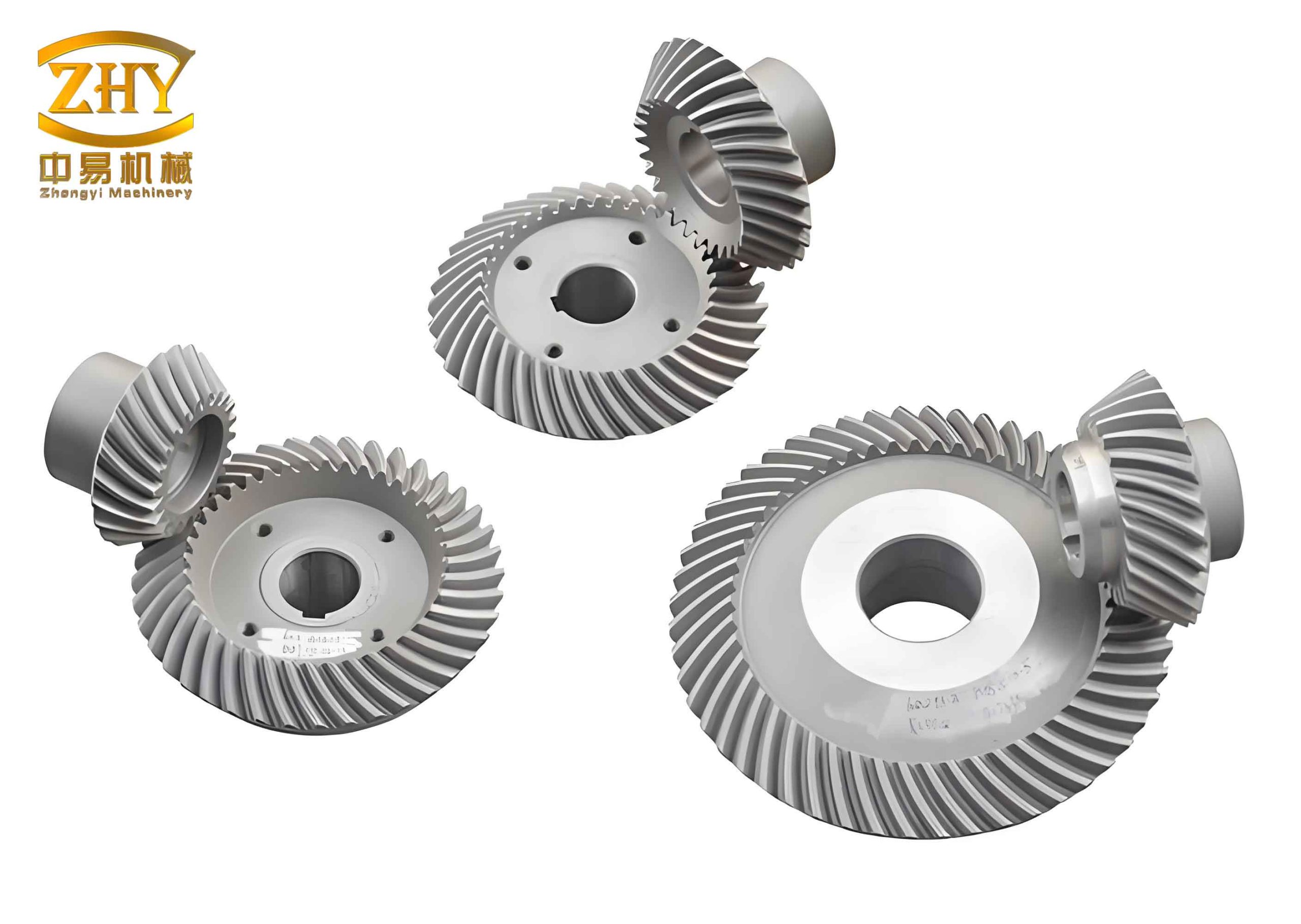
1. Theoretical Foundation: Meshing and Singularities
The generation of a gear tooth surface, such as that of a hypoid pinion, can be described as the envelope of a series of positions of a tool surface (the cutter head) relative to the workpiece. The fundamental condition for conjugation is the meshing equation, which states that the relative velocity vector at the point of contact between the two surfaces must be orthogonal to the common normal vector. For surfaces \( \Sigma^{(1)} \) (the tool) and \( \Sigma^{(2)} \) (the generated gear), this is expressed as:
$$
\vec{v}^{(12)} \cdot \vec{n} = 0
$$
where \( \vec{v}^{(12)} \) is the relative velocity and \( \vec{n} \) is the unit normal vector to the surface at the contact point.
However, to investigate the occurrence of singularities like undercutting (where the generated surface develops a cusp or edge), one must examine conditions beyond the basic meshing equation. In the theory of gearing, a “first-order” singularity, or a limiting point, occurs on the envelope surface. Research in this field establishes that such singular points satisfy both the meshing equation and an additional critical condition:
$$
\Phi = \vec{q} \cdot \vec{n} + \vec{a} \cdot \vec{v}^{(12)} = 0
$$
Here, \( \Phi \) is defined as the checking function. The vector \( \vec{q} \) is related to the derivative of the normal vector, and \( \vec{a} \) involves the relative acceleration and curvature properties. This function \( \Phi \) effectively divides the generating surface into regions. For a valid, non-undercut generation, the sign of \( \Phi \) must be consistent with the direction of the surface normal relative to the material side. If we define the normal vector \( \vec{n}^{(1)} \) of the generating tool surface \( \Sigma^{(1)} \) as pointing from the material (solid) side towards the void (empty) side, then to avoid curvature interference (undercut) on the generated surface, the condition \( \Phi < 0 \) must hold. Conversely, if the normal is defined from the void to the material, the requirement is \( \Phi > 0 \). The locus where \( \Phi = 0 \) represents the boundary of undercutting; at these points, the induced curvature becomes infinite, and the envelope surface develops a sharp edge. Therefore, monitoring the sign of the \( \Phi \) function across the potential contact lines during the generation process provides a direct criterion for undercut prediction in hyperboloid gear manufacturing.
2. Mathematical Model of the Pinion Tooth Surface
2.1 Coordinate Systems and Cutter Geometry
The generation of a hypoid pinion is typically performed using a tilted cutter head method. To formulate the tooth surface equation, a series of coordinate systems are established. The primary machine coordinate system \( \{ O’; \vec{i}_1, \vec{j}_1, \vec{k}_1 \} \) is defined at the machine center \( O’ \), with the \( \vec{i}_1-\vec{j}_1 \) plane representing the machine plane. The initial cutter vector \( \overrightarrow{O_0 M_0} \) has a magnitude equal to the cutter point radius \( r_{01} \).
The geometry of the cutter blade is crucial. For a straight-sided blade with a tip corner radius \( r_c \) and pressure angle \( \alpha \), the transition point \( M_a \) from the straight flank to the tip fillet is located at a distance \( b_r’ \) from the cutter tip point \( M_T \). This distance is given by:
$$
b_r’ = r_c \cdot \cot\left(\frac{45^\circ + \alpha/2}{2}\right) = r_c \cdot \frac{1 – \sin \alpha}{\cos \alpha}
$$
Undercut, if it occurs, will often initiate in the region generated by this tip fillet. The surface of the cutter blade cone (or plane) can be parameterized. For a specific blade section determined by the swivel angle \( \theta_1 \), the position vector \( \vec{r}_0 \) of a point on the cutter surface relative to \( O_0 \), its unit tangent vector \( \vec{t}_1 \) along the cutting direction, and its unit normal vector \( \vec{n}_1 \) can be expressed as functions of the basic machine setting angles (tilt angle \( i \), swivel angle \( \theta_1 \), and rotational position angle \( q_1 \)) and the blade pressure angle \( \alpha_{01} \):
$$
\begin{aligned}
\vec{r}_0 &= r_{01} \left[ \cos i \sin(q_1 – j) \cos\theta_1 – \sin\theta_1 \cos(q_1 – j) \right] \vec{i}_1 \\
&\quad – r_{01} \left[ \cos i \cos(q_1 – j) \cos\theta_1 + \sin\theta_1 \sin(q_1 – j) \right] \vec{j}_1 \\
&\quad + r_{01} \sin i \cos\theta_1 \vec{k}_1 \\[6pt]
\vec{t}_1 &= \left[ \cos\theta_1 \sin(\alpha_{01} – i) \sin(q_1 – j) – (1-\cos\theta_1)\cos\alpha_{01} \sin i \sin(q_1 – j) – \sin\theta_1 \sin\alpha_{01} \cos(q_1 – j) \right] \vec{i}_1 \\
&\quad + \left[ -\cos\theta_1 \sin(\alpha_{01} – i) \cos(q_1 – j) – (1-\cos\theta_1)\cos\alpha_{01} \sin i \cos(q_1 – j) + \sin\theta_1 \sin\alpha_{01} \sin(q_1 – j) \right] \vec{j}_1 \\
&\quad + \left[ \cos\theta_1 \cos(\alpha_{01} – i) + \cos\alpha_{01} \cos i (1-\cos\theta_1) \right] \vec{k}_1 \\[6pt]
\vec{n}_1 &= \left[ \cos\theta_1 \cos(\alpha_{01} – i) \sin(q_1 – j) + \sin\alpha_{01} \sin i \sin(q_1 – j)(1-\cos\theta_1) – \sin\theta_1 \cos\alpha_{01} \cos(q_1 – j) \right] \vec{i}_1 \\
&\quad + \left[ -\cos\theta_1 \cos(\alpha_{01} – i) \cos(q_1 – j) – \sin\alpha_{01} \sin i \cos(q_1 – j)(1-\cos\theta_1) – \sin\theta_1 \cos\alpha_{01} \sin(q_1 – j) \right] \vec{j}_1 \\
&\quad + \left[ -\cos\theta_1 \sin(\alpha_{01} – i) – \sin\alpha_{01} \cos i (1-\cos\theta_1) \right] \vec{k}_1
\end{aligned}
$$
2.2 The Generation Motion and Meshing Equation
The position vector of a cutter point relative to the machine origin \( O’ \) is:
$$
\vec{r}_{01} = \overrightarrow{O’O_0} + \vec{r}_0 = s_1 \cos q_1 \vec{i}_1 + s_1 \sin q_1 \vec{j}_1 + \vec{r}_0
$$
where \( s_1 \) is the radial setting distance from \( O’ \) to \( O_0 \). The relative velocity \( \vec{v}^{‘(12)} \) between the generating gear (cutter head) and the workpiece (pinion) is composed of two parts: the velocity due to the relative angular motion \( \vec{\omega}^{‘(12)} \) and the velocity due to the radial feed motion \( \dot{s}_1 \vec{t}_1 \). Additionally, the generating gear often has an eccentric mounting \( \vec{p}_1 \) which introduces a component related to the pinion’s angular speed \( d\phi_1/dt \). Thus:
$$
\vec{v}^{‘(12)} = \vec{\omega}^{‘(12)} \times \vec{r}_{01} + \dot{s}_1 \vec{t}_1 – \frac{d\phi_1}{dt} \vec{p}_1 \times \vec{m}_1
$$
Here, \( \vec{m}_1 \) is the vector from the origin to the pinion’s design crossing point. Substituting this velocity into the meshing equation \( \vec{v}^{‘(12)} \cdot \vec{n}_1 = 0 \) allows us to solve for the parameter \( \dot{s}_1 \), which is found to be a function of the basic parameters \( q_1 \) and \( \theta_1 \):
$$
\dot{s}_1 = \frac{(\vec{\omega}^{‘(12)}, \vec{r}_{01}, \vec{n}_1) – \frac{d\phi_1}{dt} (\vec{p}_1, \vec{m}_1, \vec{n}_1)}{(\vec{\omega}^{‘(12)}, \vec{t}_1, \vec{n}_1)}
$$
The notation \( (\vec{a}, \vec{b}, \vec{c}) \) represents the scalar triple product \( \vec{a} \cdot (\vec{b} \times \vec{c}) \).
2.3 Equation of the Generated Pinion Tooth Surface
Finally, the equation of the pinion tooth surface \( \vec{r}_1 \) in the machine coordinate system (later transformed to the pinion coordinate system) is given by the sum of the position vector to the cutter point, the radial feed motion, and the offset to the crossing point:
$$
\vec{r}_1 = \vec{r}_{01} + s_1 \vec{t}_1 + \vec{m}_1
$$
The surface is thus defined by the parameters \( \theta_1 \) (defining the cutter blade section) and \( q_1 \) (defining the rotational position during generation). For a fixed \( \theta_1 \), varying \( q_1 \) traces a curve on the pinion tooth surface, known as a \( \Delta q_1 \) curve.
3. Methodology for Undercut Checking in Hyperboloid Gears
The developed mathematical model enables a systematic procedure to check for undercut across the entire active profile of the hypoid pinion. The core of the procedure is the evaluation of the checking function \( \Phi \) defined in Section 1, with its terms adapted to the specific kinematics of the hypoid generator.
The term \( \vec{q} \cdot \vec{n}_1 \) in the checking function can be expanded and calculated based on the generator kinematics and surface geometry. One derived form useful for computation is:
$$
\vec{q} \cdot \vec{n}_1 = (\vec{k}_1 \times \vec{r}_{C1}) \cdot (\vec{n}_1 \times \vec{\omega}^{‘(12)}) + (\vec{\gamma}^{‘(12)}, \vec{k}_1, \vec{n}_1)
$$
where \( \vec{r}_{C1} \) is a position vector related to the cutter geometry and \( \vec{\gamma}^{‘(12)} \) is related to the angular acceleration. The vector \( \vec{a} \) is given by:
$$
\vec{a} = A_{01} \vec{v}^{‘(12)} + \vec{\omega}^{‘(12)} \times \vec{n}_1
$$
Here, \( A_{01} \) represents the normal curvature of the cutter surface at point \( M \) in the direction of \( \vec{t}_1 \times \vec{n}_1 \).
Procedure for Undercut Analysis:
- Parameter Selection: For a given hyperboloid gear design with proposed tooth height parameters (working depth coefficient \( K \) and addendum coefficient \( f_a \)), define the basic gear geometry (number of teeth \( z_1, z_2 \), offset \( E \), pitch diameters, spiral angle \( \beta \), cutter radius \( r_c \), etc.) and all machine settings (tilt \( i \), swivel \( j \), radial distance \( s_1 \), etc.).
- Profile Discretization: Discretize the tooth profile by selecting a series of constant \( \theta_1 \) values across the intended face width (e.g., \( \theta_1 = 52^\circ, 54^\circ, 56^\circ, \dots \)). Each \( \theta_1 \) defines a specific cutting plane or blade section.
- Checking Point Identification: Along each constant \( \theta_1 \) curve, identify the critical point corresponding to the transition from the straight flank to the tip fillet on the cutter. This is done by setting the radial parameter \( s_1 \) equal to the calculated distance \( b_r’ \) (Eq. 10).
- Evaluation of the Checking Function \( \Phi \): For this critical point (\( s_1 = b_r’ \)), and while satisfying the meshing equation, vary the generation rotation parameter \( q_1 \) and compute the value of the checking function \( \Phi = \vec{q} \cdot \vec{n}_1 + \vec{a} \cdot \vec{v}^{‘(12)} \).
- Interference Criterion Application:
- For the concave side of the pinion tooth: The generating surface’s normal \( \vec{n}_1 \) points from the pinion material (solid) to the void. To avoid undercut (curvature interference), the condition must be \( \Phi < 0 \). If \( \Phi > 0 \), undercut is predicted.
- For the convex side of the pinion tooth: The generating surface’s normal \( \vec{n}_1 \) points from the void to the material. To avoid undercut, the condition must be \( \Phi > 0 \). If \( \Phi < 0 \), undercut is predicted.
- Determination of Safe Addendum: Iterate the design process by adjusting the addendum coefficient \( f_a \) until, for all checked \( \theta_1 \) sections across the face width, the sign condition for \( \Phi \) is satisfied, indicating a non-undercutting design for the chosen working depth \( K \).
A critical observation from applying this methodology is the inherent asymmetry between the concave and convex sides of a hyperboloid gear pinion. The concave side is consistently more susceptible to undercutting. The limiting curve (where \( \Phi = 0 \)) for the concave side is found at a significantly lower addendum (or higher \( q_1 \) value) than that for the convex side. This means that for a given design, undercut will always manifest on the concave flank first. Therefore, the undercut check can be primarily focused on the concave side, with the convex side posing a much lower risk.
4. Design Application and Computational Results
To validate the proposed methodology, it is applied to a specific hypoid gear set. The basic geometric parameters are listed in the table below:
| Parameter | Symbol | Value |
|---|---|---|
| Pinion Teeth | \( z_1 \) | 9 |
| Gear Teeth | \( z_2 \) | 41 |
| Gear Face Width | \( b_2 \) | 33 mm |
| Offset | \( E \) | 30 mm |
| Gear Pitch Diameter | \( d_2 \) | 202 mm |
| Cutter Radius | \( r_c \) | 95.25 mm |
| Mean Spiral Angle | \( \beta_{m1} \) | 50° |
The objective is to determine the maximum allowable addendum coefficient \( f_a \) for two different working depth coefficients \( K \): a standard value of 3.9 and a high-ratio value of 4.2. The checking procedure is performed for multiple profile points (\( \theta_1 \) values). The computed values of the checking function \( \Phi \) for the concave side at the critical fillet point are summarized in the following table. The calculation seeks the smallest \( q_1 \) (most critical meshing position) for a given \( \theta_1 \) and \( f_a \). A negative \( \Phi \) indicates a safe condition (no undercut), while a positive \( \Phi \) signals potential undercut.
| Working Depth Coeff. \( K \)** | Profile Point \( \theta_1 \) (deg)** | Addendum Coeff. \( f_a \)** | Checking Function \( \Phi \) at Critical \( q_1 \)** | |
|---|---|---|---|---|
| \( q_1 \) (deg)** | \( \Phi \)** | |||
| 3.9 (Standard) | 52 | 0.17 | -5.18 | -1.957095 |
| 0.18 | -5.35 | 0.295529 | ||
| 54 | 0.19 | -3.10 | -0.490197 | |
| 0.20 | -3.28 | 1.434832 | ||
| 56 | 0.20 | -0.74 | -0.492927 | |
| 0.21 | -0.90 | 1.120926 | ||
| 58 | 0.20 | 1.8 | -0.528455 | |
| 0.21 | 1.63 | 1.463194 | ||
| 60 | 0.19 | 4.2 | -0.098588 | |
| 0.20 | 4.05 | 1.223538 | ||
| 61 | 0.17 | 5.6 | -1.083900 | |
| 0.18 | 5.44 | 0.019396 | ||
| 4.2 (High-Ratio) | 52 | 0.21 | -4.76 | -0.468006 |
| 0.22 | -5.21 | 0.000147 | ||
| 54 | 0.22 | -2.45 | -0.512098 | |
| 0.23 | -2.65 | 1.602125 | ||
| 56 | 0.23 | -0.09 | -0.394014 | |
| 0.24 | -0.30 | 1.698809 | ||
| 58 | 0.22 | 2.50 | -0.780170 | |
| 0.23 | 2.34 | 0.713620 | ||
| 60 | 0.22 | 5.28 | -0.929905 | |
| 0.23 | 5.14 | 0.287953 | ||
| 61 | 0.21 | 6.75 | -0.898752 | |
| 0.22 | 6.62 | 0.001164 | ||
Analysis of Results:
- For \( K = 3.9 \), an addendum coefficient \( f_a = 0.17 \) yields negative \( \Phi \) values across all profile points, indicating a safe design. Increasing \( f_a \) to 0.18 causes \( \Phi \) to become positive at several points (\( \theta_1 = 52^\circ, 56^\circ, 58^\circ, 60^\circ, 61^\circ \)), signaling undercut risk.
- For the high-ratio design with \( K = 4.2 \), the safe addendum is lower. The coefficient \( f_a = 0.21 \) is safe, while \( f_a = 0.22 \) leads to positive \( \Phi \) (undercut risk) at all checked profile points.
- The table clearly shows that the critical, most limiting profile point shifts depending on the design (e.g., near \( \theta_1 = 52^\circ \) for \( K=3.9 \), \( f_a=0.18 \), and near \( \theta_1 = 61^\circ \) for \( K=4.2 \), \( f_a=0.22 \)). A complete check must therefore span the entire active profile.
- It is important to note a practical consideration: computationally predicted undercut with a very small positive \( \Phi \) value (e.g., 0.000147) may not manifest as a physically observable or detrimental root cutting in the actual machining process due to tool edge rounding and machine elasticity. Thus, a small positive margin might be acceptable, but it requires experimental verification.
To conclusively validate the method, a physical hypoid pinion was manufactured using the high-ratio parameters \( K=4.2 \) and the predicted safe addendum \( f_a=0.21 \). The cutting test resulted in a clean tooth form with no visible undercut, confirming the accuracy and practical utility of the proposed analytical checking methodology for hyperboloid gear design.
5. Conclusions and Design Guidelines
This investigation into the undercutting behavior of high-ratio hypoid gears leads to several definitive conclusions and actionable guidelines for gear engineers:
- Necessity of Undercut Verification for Non-Standard Designs: When designing a hyperboloid gear set, especially one departing from standard tooth proportions (e.g., adopting a high tooth depth for increased strength or contact ratio), it is imperative to perform an undercut verification. Blindly using standard coefficient tables or extrapolating from them carries a high risk of generating a pinion with a weakened, undercut root form.
- Validity of the Checking Function Methodology: The analytical method based on the checking function \( \Phi \), derived from the fundamental principles of conjugate surface generation, provides a reliable and general-purpose tool for undercut prediction. It successfully identifies the critical relationship between the working depth coefficient \( K \), the addendum coefficient \( f_a \), and the machine kinematics specific to hyperboloid gear generation.
- Asymmetry in Undercut Susceptibility: A fundamental characteristic of hypoid and similar offset gear geometries is the pronounced asymmetry in undercut risk. The concave (drive side for a typical automotive pinion) flank is far more prone to undercutting than the convex flank. Therefore, the root cause of failure in over-ambitious high-ratio designs will invariably be undercut on the concave side. The design check can be prioritized accordingly.
- Design Procedure for High-Ratio Hyperboloid Gears:
- Step 1: Define the basic gear set geometry (ratios, offset, spiral angle, etc.) and the desired increased working depth coefficient \( K \).
- Step 2: Establish all necessary machine-tool settings for pinion generation using standard hypoid gear design software or methods.
- Step 3: Implement the undercut checking algorithm. Discretize the tooth profile into multiple sections (constant \( \theta_1 \)). For each section, at the critical cutter tip transition point (\( s_1 = b_r’ \)), compute the checking function \( \Phi \) while satisfying the meshing equation.
- Step 4: Iteratively adjust the pinion addendum coefficient \( f_a \) until the condition \( \Phi < 0 \) is satisfied for all profile sections on the concave side. This yields the maximum safe addendum for the chosen depth \( K \).
- Step 5: Verify the convex side if desired (it will almost certainly be safe). Finally, validate the design through a prototype cutting test.
In summary, the pursuit of advanced performance through high-ratio tooth designs in hyperboloid gears is a viable path, but it must be navigated with careful analytical support. The methodology presented here, centered on a rigorously defined checking function, empowers designers to push the boundaries of tooth geometry while maintaining the integrity of the gear root, ensuring both the strength and quiet operation expected of modern hypoid gear drives.