
In the field of gear manufacturing, the precision finishing of hyperboloid gears is a critical process that ensures optimal performance in applications such as automotive differentials and industrial machinery. Traditionally, grinding has been used for hard-faced hyperboloid gears, but it is often expensive and requires specialized equipment. As an alternative, shaving with carbide tools has emerged as a viable method, offering cost-effectiveness and improved efficiency. In this article, I will delve into the computational aspects of shaving for hyperboloid gears, focusing on the changes in cutting principles due to carbide shavers and the precise calculation of tool parameters. The methodology presented here enables accurate shaving calculations, enhancing the quality and productivity of hyperboloid gear production.
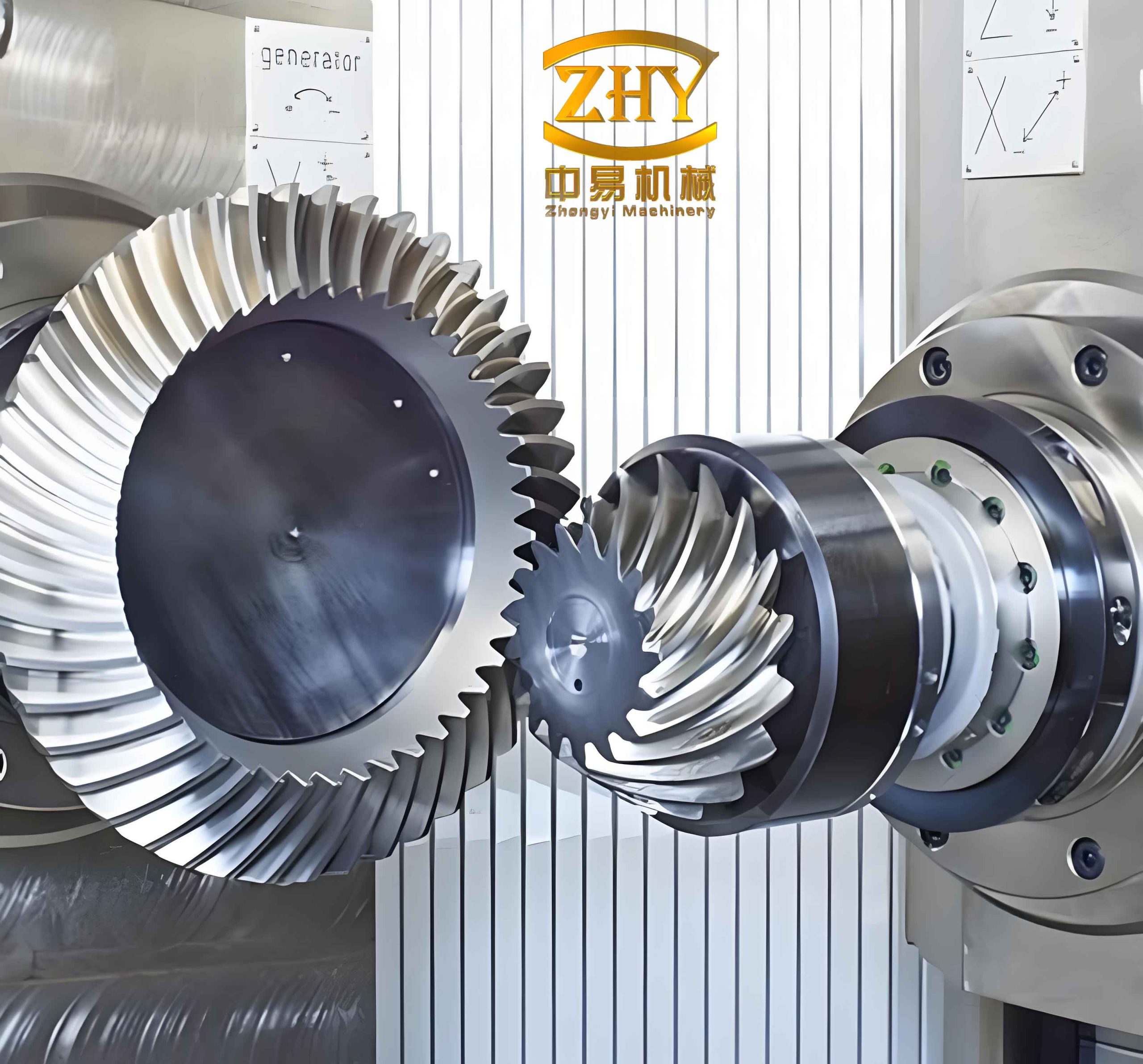
Hyperboloid gears, also known as hypoid gears, are characterized by their skewed axes and complex tooth geometry, which allow for smooth torque transmission and high load capacity. The shaving process involves using a carbide cutter with a negative rake angle and straight cutting edges, which alters the tool’s generating surface compared to conventional high-speed steel cutters. This shift necessitates a revised approach to cutting theory, as the generating surface transforms from a conical shape to a hyperboloid of one sheet. I will explore this transformation in detail, deriving the equations for the shaving tool’s generating surface and subsequently applying them to cutting calculations. Throughout this discussion, the term hyperboloid gears will be emphasized to underscore the specific gear type under consideration.
The fundamental change in the shaving process for hyperboloid gears lies in the tool’s generating surface. For a conventional high-speed steel cutter, the generating surface is a cone with a tool profile angle, denoted as $\alpha$. However, with carbide shavers, the cutting edge is a straight line inclined at a negative rake angle $\lambda_G$, passing through a conjugate contact point $M$ on the gear tooth surface. This configuration results in a generating surface that is a hyperboloid of revolution. To formulate this, I establish two coordinate systems: $\Sigma$ and $\Sigma_n$, where the $k$-axis aligns with the original conical surface’s axis, and the $i$-axis passes through the original tool tip $P$. In $\Sigma_n$, the equation of the cutting edge is given by:
$$ \vec{r}^{(n)}_c = \begin{pmatrix} 0 \\ a \sin \lambda_G \\ -a \cos \lambda_G \end{pmatrix} $$
Transforming this into the $\Sigma$ system, the coordinates become:
$$ \vec{r}_c = \begin{pmatrix} R_c – (b – a \cos \lambda) \sin \alpha \\ a \cos \lambda \\ (b – a \cos \lambda) \cos \alpha \end{pmatrix} $$
Here, $R_c$ is the tool tip radius, $b = MP$ is derived from conventional cutting calculations, and $\alpha$ is the tool profile angle (positive for internal cutters and negative for external cutters). Since the cutting edge and tool axis are skew lines, the generating surface formed by rotating the edge around the axis is a hyperboloid. Let $\theta$ be the initial rotation angle of the cutting edge around the tool axis. The generating surface equation for the shaving tool is:
$$ \vec{r}_d = \vec{r}_d(a, \theta) = \begin{pmatrix} \sqrt{r_{cx}^2 + r_{cy}^2} \cdot \cos \theta \\ \sqrt{r_{cx}^2 + r_{cy}^2} \cdot \sin \theta \\ r_{cz} \end{pmatrix} $$
To analyze the surface properties, I compute the partial derivatives with respect to $a$ and $\theta$. Define $q = \sqrt{r_{cx}^2 + r_{cy}^2}$ and $p = r_{cx} \frac{dr_{cx}}{da} + r_{cy} \frac{dr_{cy}}{da}$. Then:
$$ \vec{r}_{da} = \begin{pmatrix} \frac{p \cos \theta}{q} \\ \frac{p \sin \theta}{q} \\ -\cos \lambda \cos \alpha \end{pmatrix} $$
$$ \vec{r}_{d\theta} = \begin{pmatrix} -q \sin \theta \\ q \cos \theta \\ 0 \end{pmatrix} $$
The normal vector to the hyperboloid surface is given by the cross product:
$$ \vec{r}_{da} \times \vec{r}_{d\theta} = \begin{pmatrix} q \cos \lambda \cos \alpha \cos \theta \\ q \cos \lambda \cos \alpha \sin \theta \\ p \end{pmatrix} $$
At the conjugate contact point $M$, where $\theta = 0$ and $a = 0$, the normal vector simplifies to:
$$ \vec{n}_M = \begin{pmatrix} (R_c – b \sin \alpha) \cos \lambda \cos \alpha \\ 0 \\ (R_c – b \sin \alpha) \cos \lambda \sin \alpha \end{pmatrix} $$
For the original conical generating surface, the normal vector at $M$ is:
$$ \vec{n} = \begin{pmatrix} \cos \alpha \\ 0 \\ \sin \alpha \end{pmatrix} $$
These vectors are proportional, indicating that the hyperboloid and conical surfaces share the same normal at $M$, and the coordinate plane $j_n M k_n$ is their common tangent plane. From differential geometry, the curvature lines of a hyperboloid of revolution are circles and hyperbolas, so both surfaces have identical principal directions at $M$. This allows the use of conical surface methods to compute the gear tooth surface’s normal and tangent vectors, facilitating the transition to shaving calculations for hyperboloid gears.
The first fundamental quantities of the shaving tool generating surface are:
$$ E = \vec{r}_{da}^2, \quad F = \vec{r}_{da} \cdot \vec{r}_{d\theta}, \quad G = \vec{r}_{d\theta}^2 $$
The surface normal vector is:
$$ \vec{n} = \frac{\vec{r}_{da} \times \vec{r}_{d\theta}}{\sqrt{EG – F^2}} $$
At point $M$, this aligns with the conical surface normal. By Meusnier’s theorem, the principal curvature in the circular direction is:
$$ k_1 = -\frac{\cos \alpha}{R_c – b \sin \alpha} $$
Since the cutting edge direction is an asymptotic direction on the generating surface (where the normal curvature is zero), Euler’s formula yields the principal curvature in the hyperbolic direction:
$$ k_2 = \frac{\tan^2 \lambda \cos \alpha}{R_c – b \sin \alpha} $$
These curvatures are essential for subsequent cutting calculations. In shaving hyperboloid gears, the tool parameters must be adjusted to account for the hyperboloid generating surface. The following table summarizes key parameters involved in the shaving process for hyperboloid gears:
| Parameter | Symbol | Description | Typical Value Range |
|---|---|---|---|
| Tool Tip Radius | $R_c$ | Radius at the cutting edge tip | 50–200 mm |
| Tool Profile Angle | $\alpha$ | Angle of the tool profile | ±20° |
| Negative Rake Angle | $\lambda_G$ | Inclination of the cutting edge | -5° to -15° |
| Conjugate Contact Point | $M$ | Point on gear tooth surface | Varies with design |
| Principal Curvature (Circular) | $k_1$ | Curvature in circular direction | Negative value |
| Principal Curvature (Hyperbolic) | $k_2$ | Curvature in hyperbolic direction | Positive value |
Moving to the cutting calculations for hyperboloid gears, the first and second-order parameters of the gear tooth surface are derived based on the relative motion between the tool and workpiece. Using Baxter’s formula, the second-order parameters—such as normal curvatures and geodesic torsion—at point $M$ on the gear tooth surface can be determined. For the pinion (small gear) tooth surface, let the corrected normal curvatures and geodesic torsion at the conjugate point be $k_{xc}$, $k_{yc}$, and $G_c$, respectively. The relationship between induced normal curvatures and geodesic torsion is given by:
$$ (k_{xc} – k_{xd})(k_{yc} – k_{yd}) = G_c^2 $$
Here, $k_{xd}$ and $k_{yd}$ are the first and second principal curvatures of the shaving tool generating surface for the pinion. Similarly, for the pinion tool, $k_{yd} = -k_{xd} \tan^2 \lambda_p$, where $\lambda_p$ is the rake angle for the pinion shaving tool. Substituting this into the equation yields:
$$ k_{xd} = \frac{Q \pm \sqrt{Q^2 – 4 \tan^2 \lambda_p (G_c^2 – k_{xc} k_{yc})}}{2 \tan^2 \lambda_p} $$
where $Q = k_{xc} \tan^2 \lambda_p – k_{yc}$. From Euler’s and Bertrand’s formulas in differential geometry, we have:
$$ k_{xc} = k_1 \cos^2 \phi + k_2 \sin^2 \phi $$
$$ k_{yc} = k_1 \sin^2 \phi + k_2 \cos^2 \phi $$
$$ G_c = (k_2 – k_1) \sin \phi \cos \phi $$
This leads to $G_c^2 – k_{xc} k_{yc} = -k_1 k_2 = -K$, where $K$ is the total curvature at that point on the tooth surface. Thus, the expression simplifies to:
$$ k_{xd} = \frac{-b \pm \sqrt{b^2 + 4 \tan^2 \lambda_p K}}{2 \tan^2 \lambda_p} $$
According to the cutting calculation conventions, the normal vector direction for the pinion convex surface points inward toward the tooth material, while for the concave surface, it points outward. This implies $k_{xd} > 0$ for convex surfaces. Since the convex surface of a hyperboloid gear is an elliptic point ($K > 0$), the negative sign in the square root is invalid. Therefore, for the pinion convex tool:
$$ k_{xd} = \frac{k_{xc} \tan^2 \lambda_p – k_{yc} + \sqrt{(k_{xc} \tan^2 \lambda_p – k_{yc})^2 + 4K \tan^2 \lambda_p}}{2 \tan^2 \lambda_p} $$
Using Meusnier’s theorem, the required tool tip radius for the pinion is:
$$ r_{cp} = \frac{\cos \alpha_{bp}}{k_{xd}} – b_p \sin \alpha_{bp} $$
Here, $b_p$ is obtained from conventional calculations, and $r_{cp}$ is rounded to a standard tool size. For the pinion concave surface, an appropriate tool size is selected based on practical considerations. Other tool parameters and machine adjustments follow standard cutting calculations for hyperboloid gears.
To illustrate the computational flow for shaving hyperboloid gears, I present a step-by-step algorithm that integrates the derived equations. This algorithm ensures precise parameter determination, which is crucial for achieving desired contact patterns and tooth geometry in hyperboloid gears.
- Input Initial Parameters: Define gear geometry, tool specifications, and cutting conditions for hyperboloid gears.
- Compute Conjugate Point: Calculate the coordinates of point $M$ using conventional gear meshing theory.
- Determine Generating Surface: Derive the hyperboloid generating surface equations based on tool rake angle and profile.
- Calculate Curvatures: Compute principal curvatures $k_1$ and $k_2$ for the tool surface at $M$.
- Adjust for Pinion: Apply the corrected normal curvatures and geodesic torsion for pinion tooth surfaces.
- Solve for Tool Parameters: Use the equations to find $k_{xd}$ and subsequently $r_{cp}$ for convex and concave surfaces.
- Validate and Iterate: Check results against design tolerances and iterate if necessary for hyperboloid gears.
The effectiveness of this methodology is evident in its ability to handle the complexities of hyperboloid gears, where traditional grinding is replaced by shaving. By accurately modeling the hyperboloid generating surface, the shaving process can achieve comparable precision at a lower cost. The table below compares key aspects of grinding and shaving for hyperboloid gears, highlighting the advantages of the shaving approach:
| Aspect | Grinding | Shaving (Carbide Tool) |
|---|---|---|
| Cost | High due to equipment and abrasives | Lower, utilizing durable carbide tools |
| Precision | Very high, suitable for critical applications | High, with proper parameter calculation |
| Tool Life | Short, frequent dressing required | Long, thanks to carbide hardness |
| Surface Finish | Excellent, minimal roughness | Good, dependent on tool geometry |
| Applicability | Limited to high-precision hyperboloid gears | Broad, for most industrial hyperboloid gears |
In practice, the shaving process for hyperboloid gears involves iterative adjustments to optimize tooth contact and noise reduction. The derived equations allow for simulation-based tuning, reducing trial-and-error on the shop floor. For instance, by varying the rake angle $\lambda_G$, one can influence the tool’s generating surface and thus the tooth surface curvature. This flexibility is particularly beneficial for custom hyperboloid gears used in specialized machinery.
Furthermore, the integration of computer-aided design (CAD) software enhances the calculation process. Using numerical methods, the hyperboloid generating surface can be discretized and analyzed for multiple points along the tooth flank. This enables a comprehensive evaluation of the shaving process across the entire gear tooth, ensuring consistency for hyperboloid gears. The following formula set encapsulates the core equations for shaving calculation, serving as a quick reference for engineers working on hyperboloid gears:
$$ \text{Generating Surface: } \vec{r}_d = \begin{pmatrix} \sqrt{r_{cx}^2 + r_{cy}^2} \cos \theta \\ \sqrt{r_{cx}^2 + r_{cy}^2} \sin \theta \\ r_{cz} \end{pmatrix} $$
$$ \text{Principal Curvatures: } k_1 = -\frac{\cos \alpha}{R_c – b \sin \alpha}, \quad k_2 = \frac{\tan^2 \lambda \cos \alpha}{R_c – b \sin \alpha} $$
$$ \text{Pinion Tool Curvature: } k_{xd} = \frac{k_{xc} \tan^2 \lambda_p – k_{yc} + \sqrt{(k_{xc} \tan^2 \lambda_p – k_{yc})^2 + 4K \tan^2 \lambda_p}}{2 \tan^2 \lambda_p} $$
$$ \text{Tool Tip Radius: } r_{cp} = \frac{\cos \alpha_{bp}}{k_{xd}} – b_p \sin \alpha_{bp} $$
Looking ahead, advancements in materials and manufacturing technologies may further refine the shaving process for hyperboloid gears. For example, the development of coated carbide tools could enhance wear resistance, extending tool life and maintaining accuracy over longer production runs. Additionally, real-time monitoring systems could be integrated to adjust shaving parameters dynamically, adapting to variations in gear blanks or tool wear. These innovations will continue to make shaving an attractive option for finishing hyperboloid gears, balancing cost and performance.
In conclusion, the calculation methodology for shaving hyperboloid gears presented here provides a robust framework for transitioning from grinding to carbide-based shaving. By accounting for the hyperboloid generating surface and deriving precise tool parameters, manufacturers can achieve high-quality gear teeth with improved efficiency. The emphasis on hyperboloid gears throughout this discussion underscores the specificity of the approach, ensuring applicability to this complex gear type. As industry demands for cost-effective and precise gear manufacturing grow, such computational methods will play a pivotal role in optimizing production processes for hyperboloid gears.