
The precise meshing behavior of hyperboloid gears is a cornerstone of modern automotive and industrial drivetrain design. Ensuring smooth power transmission, minimal noise, and high durability requires a deep understanding of how the gear teeth interact throughout the entire engagement cycle. Traditional design methods focus on achieving optimal conditions at a chosen reference point on the tooth flank. However, to guarantee performance across the full path of contact and under realistic conditions of misalignment and load, a comprehensive simulation approach is indispensable. This is where Tooth Contact Analysis (TCA) comes into play. In this article, I will develop and present a complete methodology for simulating the meshing process of hyperboloid gears, encompassing both flank contact and the critical, often-overlooked phase of edge contact. This holistic approach allows for accurate computer-based prediction of gear performance, significantly reducing the need for physical prototyping and testing.
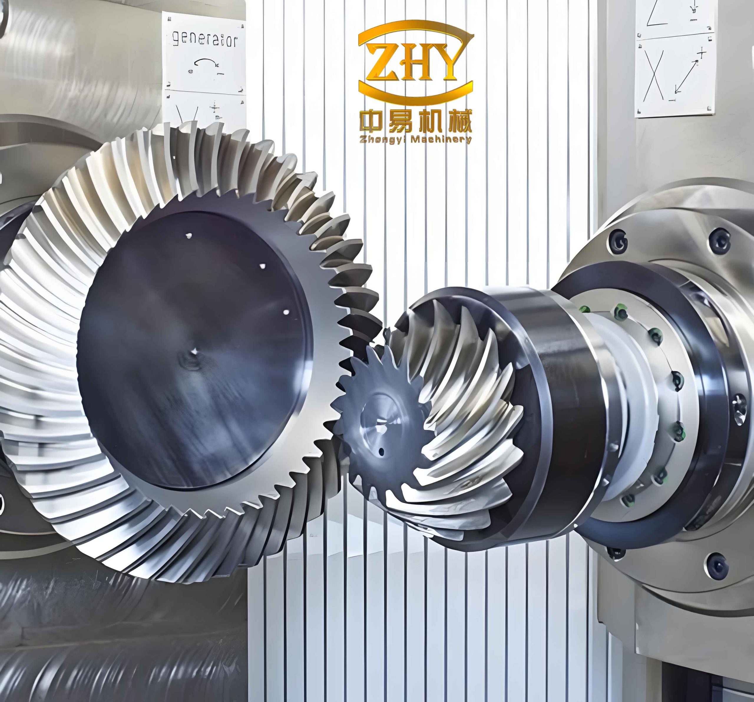
The unique geometry of hyperboloid gears, characterized by crossed axes and an offset (hypoid offset), allows for compact and versatile design configurations. However, this same complexity makes their tooth surfaces non-developable and conjugacy is not inherently guaranteed. Their flanks are generated through a simulated gear mating process using cutting tools on specialized hypoid gear generators. Therefore, a mathematical representation of the machined tooth surface is the fundamental starting point for any TCA.
We begin by modeling the gear tooth surfaces. Consider the cutting tool, typically a circular face-mill cutter, which generates the gear flank. For the gear member (often the ring gear), the cutter surface can be described in its local coordinate system \( S_c \) using two parameters: the cutter surface parameter \( \theta_G \) and the radial distance \( s_G \). A point on the cutter surface is given by:
$$
\vec{r_c}(\theta_G, s_G) = \begin{bmatrix}
(r_{c2} – s_G \sin \alpha_G) \cos \theta_G \\
(r_{c2} – s_G \sin \alpha_G) \sin \theta_G \\
-s_G \cos \alpha_G \\
1
\end{bmatrix}
$$
where \( r_{c2} \) is the cutter point radius and \( \alpha_G \) is the cutter blade pressure angle. The unit normal vector to the cutter surface is:
$$
\vec{n_c}(\theta_G) = \begin{bmatrix}
-\cos \alpha_G \cos \theta_G \\
-\cos \alpha_G \sin \theta_G \\
-\sin \alpha_G
\end{bmatrix}
$$
This cutter surface must then be mapped onto the gear blank through the kinematics of the gear generation machine. This involves a series of coordinate transformations from the cutter system \( S_c \) to the machine tool system and finally to the coordinate system \( S_2 \) rigidly connected to the gear. The transformation accounts for the machine settings: the cutter radial setting \( S_{rG} \), the angle of the cradle \( \psi_{cG} \), the rotation of the gear blank \( \phi_{2G} \), and the basic machine root angle \( \gamma_{mG} \). The generated gear surface \( \vec{r}_2 \) in \( S_2 \) is a function of the surface parameters and the machine kinematics:
$$
\vec{r}_2(\theta_G, s_G, \phi_{2G}) = [M_{2m}][M_{mc}(\psi_{cG})][M_{c0}][M_{0c}(\phi_c)]\vec{r_c}(\theta_G, s_G)
$$
During the generation process, the cutter and the gear blank are in a simulated meshing condition, enforced by the equation of meshing:
$$
f(\theta_G, s_G, \phi_{2G}) = \vec{n} \cdot \vec{v}^{(c2)} = 0
$$
where \( \vec{v}^{(c2)} \) is the relative velocity between the cutter and the gear. This equation implicitly defines a relationship \( s_G = s_G(\theta_G, \phi_{2G}) \). By solving this equation and substituting back, we can represent the gear tooth surface as a two-parameter family in the gear coordinate system: \( \vec{r}_2 = \vec{r}_2(\theta_G, \phi_{2G}) \), with its corresponding normal \( \vec{n}_2 \). A completely analogous procedure is followed to derive the mathematical model for the pinion tooth surface \( \vec{r}_1(\theta_P, \phi_{1P}) \) in its coordinate system \( S_1 \), using its specific machine settings and cutter geometry (often with a different pressure angle \( \alpha_P \)).
The core of Tooth Contact Analysis for hyperboloid gears lies in simulating the mating of these mathematically defined surfaces. We establish a fixed reference coordinate system \( S_f \) attached to the gear housing. The positioned and oriented gear and pinion surfaces in this global system are:
$$
\begin{aligned}
\vec{R}_1(\theta_P, \phi_{1P}, \phi_1) &= [M_{f1}(\phi_1)] \vec{r}_1(\theta_P, \phi_{1P}) \\
\vec{R}_2(\theta_G, \phi_{2G}, \phi_2) &= [M_{f2}(\phi_2)] \vec{r}_2(\theta_G, \phi_{2G})
\end{aligned}
$$
where \( \phi_1 \) and \( \phi_2 \) are the rotational angles of the pinion and gear during operation, and \( [M_{f1}], [M_{f2}] \) are transformation matrices incorporating the shaft angle \( \Sigma \), offset \( E \), and mounting positions.
For the two surfaces to be in contact at a given instant, they must share a common point and have a common surface normal at that point (neglecting elastic deformation for the kinematic analysis). This yields the system of contact equations:
$$
\begin{aligned}
\vec{R}_1(\theta_P, \phi_{1P}, \phi_1) &= \vec{R}_2(\theta_G, \phi_{2G}, \phi_2) \quad &\text{(Position Continuity)} \\
\vec{n}_f^{(1)}(\theta_P, \phi_{1P}, \phi_1) &= \vec{n}_f^{(2)}(\theta_G, \phi_{2G}, \phi_2) \quad &\text{(Normal Vector Collinearity)}
\end{aligned}
$$
Since \( \vec{n}_f \) is a unit vector, the second equation provides only two independent scalar equations. Thus, we have five independent scalar equations involving six unknowns: \( \theta_P, \phi_{1P}, \phi_1, \theta_G, \phi_{2G}, \phi_2 \). By choosing one parameter, typically the pinion rotation angle \( \phi_1 \), as the input, the system can be solved numerically (e.g., using Newton-Raphson method) for the remaining five unknowns. Scanning through the meshing cycle by incrementing \( \phi_1 \) provides the path of contact points on both tooth flanks.
From the contact point data, two key performance indicators are derived. First, the transmission error (TE), which is a primary source of gear noise, is calculated as the deviation of the actual gear position from its theoretical, perfectly conjugate position:
$$
\Delta \phi_2(\phi_1) = (\phi_2 – \phi_{2,0}) – \frac{N_1}{N_2} (\phi_1 – \phi_{1,0})
$$
where \( N_1, N_2 \) are the numbers of teeth, and \( \phi_{1,0}, \phi_{2,0} \) are initial reference angles. A smooth, low-amplitude TE curve is desirable. Second, the instantaneous contact ellipse is predicted. By calculating the principal curvatures and directions of both surfaces at the contact point and assuming a small, constant elastic approach (Hertzian contact theory), the size and orientation of the contact patch can be determined. This is visualized as the bearing pattern on the tooth flank.
Classical TCA, as described, models ideal flank-to-flank contact. However, in real-world applications, manufacturing errors, assembly misalignments, and deflections under load can shift the contact path towards the edge of the tooth. A sudden loss of contact at the edge in a pure flank TCA simulation suggests discontinuity, which is not physically accurate. In reality, contact transitions to the edge of one tooth sliding against the flank of the mating tooth. This edge contact phase must be analyzed to complete the simulation of the meshing process for hyperboloid gears.
Consider the case where the pinion tooth edge (e.g., the tip line) makes contact with the gear tooth flank. The edge is a curve on the pinion tooth surface, defined by a fixed relationship between its parameters, such as \( \theta_P = \text{constant} \) (for a profile edge) or a relationship like \( s_P(\theta_P) \) defining the tip line. The condition for this edge to contact the gear flank is a modification of the standard TCA equations:
$$
\begin{cases}
\vec{R}_1^{edge}(\phi_{1P}, \phi_1) = \vec{R}_2(\theta_G, \phi_{2G}, \phi_2) \\
\vec{n}_f^{(1)} \cdot \frac{\partial \vec{R}_1^{edge}}{\partial l} = 0
\end{cases}
$$
The first equation ensures a common point. The second equation is the key to edge contact: it states that the common surface normal \( \vec{n}_f^{(1)} \) (which is normal to the *gear* flank at the contact point) must be perpendicular to the tangent vector \( \frac{\partial \vec{R}_1^{edge}}{\partial l} \) of the pinion edge curve. This is because the edge can only transmit force normal to its tangent. A simpler method to obtain the edge tangent is to use the cross product of the surface normal at the edge point and the normal of the tooth tip cone surface at that point. For a pinion tip edge contact, an additional condition is that the pinion declination angle equals its tip cone angle \( \delta_{a1} \). Solving this augmented system provides the complete motion trajectory including edge contact, revealing significant changes in the transmission error and contact pattern during this transition phase.
To demonstrate the application of the complete TCA methodology for hyperboloid gears, let’s consider a numerical example. The following table outlines the basic geometric parameters of a sample hypoid gear set.
| Parameter | Pinion | Gear |
|---|---|---|
| Number of Teeth | 10 | 41 |
| Mean Spiral Angle | 54.19° | 30.37° |
| Shaft Angle \( \Sigma \) | 90° | |
| Offset \( E \) | 28.575 mm | |
| Face Width | 54.00 mm | 36.53 mm |
The final tooth form is controlled by the machine settings during cutting. Two different sets of pinion machine settings (Design A and Design B) are derived to meet specific pre-designed contact conditions at the reference point. These conditions are summarized below:
| Condition | Design A | Design B |
|---|---|---|
| Reference Point Location | 111.163 mm from apex | 111.163 mm from apex |
| Contact Ellipse Semi-Major Axis | 4.8 mm | 4.8 mm |
| Path Tangent Angle on Gear \( \zeta_2 \) | 40° | 10° |
| Transmission Error Slope \( d(\Delta \phi_2)/d\phi_1 \) | -0.001 | 0.0 |
Running the flank TCA for both designs yields distinct contact patterns and transmission error curves. Design A shows a more diagonal contact path and a linear, slightly negative slope TE curve. Design B shows a more lengthwise contact path and a parabolic TE curve with zero slope at the reference point. Both satisfy their design targets, demonstrating the control TCA provides. Now, let’s introduce a common assembly error: a 0.2 mm increase in the offset \( E \). Performing only flank TCA on Design A with this error shows the contact patch shifting sharply towards the toe and a dramatically altered, discontinuous-looking TE curve. This discontinuity is an artifact of the model lacking edge contact. When the complete TCA including edge contact is performed, the simulation reveals a smooth transition: as one pair of teeth disengages with edge contact, the next pair engages. The TE curve now shows a continuous but steeper drop during the edge-contact phase, providing a physically accurate and complete picture of the meshing performance under misalignment.
The development and implementation of a comprehensive Tooth Contact Analysis methodology, integrating both flank and edge contact simulation, is essential for the advanced design and validation of hyperboloid gears. This computational approach allows engineers to precisely predict and optimize meshing characteristics such as the contact pattern path, bearing ellipse size and orientation, and transmission error under a wide range of design parameters and anticipated operational errors. By virtually prototyping and testing hyperboloid gears in this manner, manufacturers can achieve higher performance, reduced noise and vibration, and extended gear life, while significantly shortening development cycles and lowering costs associated with physical trial-and-error methods. The ability to accurately model the entire engagement cycle, including the critical edge contact transition, makes this TCA strategy a powerful tool for mastering the complex geometry of hyperboloid gears.