
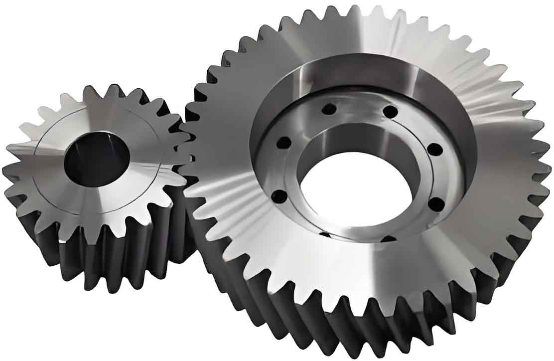
The translation of engineering design intent into a manufacturable product hinges on the precise interpretation of mechanical drawings. While traditional two-dimensional (2D) drawings comprehensively convey shape, dimensions, and critical tolerances, modern manufacturing and simulation increasingly rely on three-dimensional (3D) digital models. A significant gap exists in this transition: the loss or ambiguous representation of Geometric Dimensioning and Tolerancing (GD&T) and surface finish information in the 3D model. This paper addresses this challenge by proposing a novel, automated methodology for reconstructing a fully annotated 3D model of cylindrical gears directly from their DXF (Drawing Exchange Format) files. Our method not only extracts the geometric form but also intelligently associates and preserves key tolerance and roughness specifications.
The core of our methodology involves a multi-stage pipeline: parsing the DXF file to separate entities and annotations, clustering these elements into distinct orthographic views using the K-means algorithm, employing a Backpropagation (BP) neural network to correlate dimensions with their corresponding geometric features, and finally, driving a parametric CAD model to generate a 3D representation with integrated tolerance attributes. This approach moves beyond simple geometry reconstruction to create a semantically richer digital twin of the cylindrical gear, which is crucial for downstream applications like tolerance analysis and automated process planning.
1. The DXF File as a Data Source for Cylindrical Gears
DXF, a CAD data file format, serves as an excellent intermediary for this task. It provides a structured, text-based representation of the drawing containing distinct sections for entities (lines, circles, arcs), layers, blocks, and annotations. For reconstructing cylindrical gears, we systematically extract four key information types:
- Entity Information: The fundamental geometric primitives defining the gear’s shape—lines for keyways and profiles, circles for pitch and root diameters, and arcs for fillets.
- Annotation Information: This includes linear, diametral, radial, and angular dimensions. Each dimension object contains data on its type, leader line points, and the textual value of the dimension itself.
- Surface Finish (Roughness) Symbols: Symbols defined per standards like GB/T 131-2006 (or ISO 1302). We extract the symbol’s graphical elements and, crucially, the point where its leader line attaches to a geometric entity.
- Geometric Tolerance Symbols: Blocks containing form, orientation, and location tolerances (e.g., circular runout, symmetry). These are treated as composite graphical objects.
The extraction process involves parsing the DXF file structure, iterating through entity lists, and retrieving coordinates, layer names, and block references. For complex symbols like roughness and geometric tolerances, the graphical data within blocks is re-rendered into image snippets for subsequent pattern matching.
2. View Segmentation via K-Means Clustering
A single DXF file of a cylindrical gear typically contains entities belonging to multiple orthographic views (e.g., front, side, section). The first step in making sense of the data is to automatically cluster entities into their respective views. We achieve this using the K-means clustering algorithm, an unsupervised method ideal for partitioning data into K clusters where each entity belongs to the cluster with the nearest mean (centroid).
The process is as follows:
- Centroid Initialization: We first identify centerlines (entities on a “Center” layer). By calculating intersections between these centerlines, we obtain candidate points that often correspond to the center of circles or symmetric features in each view. These intersection points serve as the initial centroids for the K-means algorithm, where K is the number of distinct views identified.
- Feature Vector Creation: For every entity to be clustered (lines, circles, arcs, and even dimension leader points), we create a feature vector. A simple and effective vector is the geometric centroid of the entity. For a line, it’s the midpoint; for a circle or arc, it’s its center point.
- Clustering: The K-means algorithm then assigns each entity’s feature vector to the nearest centroid based on Euclidean distance, forming initial clusters. Centroids are recalculated as the mean of all points in the cluster, and the assignment process iterates until convergence. The mathematical formulation for assigning an entity with centroid \( \mathbf{x} \) to a cluster \( C_i \) with centroid \( \mathbf{\mu_i} \) is:
$$ C_i = \{ \mathbf{x}_p : \| \mathbf{x}_p – \mathbf{\mu}_i \|^2 \le \| \mathbf{x}_p – \mathbf{\mu}_j \|^2 \; \forall j, 1 \le j \le k \} $$
The centroid update rule is:
$$ \mathbf{\mu}_i = \frac{1}{|C_i|} \sum_{\mathbf{x}_p \in C_i} \mathbf{x}_p $$
This process effectively segregates the sprawling data from the DXF file into logical, view-specific groups, which is foundational for correlating dimensions in one view with geometry in another. The figure below illustrates a typical cylindrical gear drawing that serves as input to this process.
3. Feature Recognition and Parameter Mapping using BP Neural Network
With entities clustered into views, the next challenge is to interpret the drawing semantically. For a cylindrical gear, this means identifying critical parameters like addendum diameter, dedendum diameter, keyway width, web thickness, etc., from the dimension text and linking them unambiguously to the correct geometric entities. We employ a supervised machine learning approach using a Backpropagation (BP) Neural Network for this intelligent mapping.
The network is designed to learn the complex relationship between dimension presentation and its actual numeric value, which can be affected by scale factors, viewports, and drawing standards. The architecture and key formulas are detailed below:
Network Architecture & Forward Propagation:
- Input Layer: Features derived from the dimension text and its context (e.g., normalized position relative to view center, associated layer name, dimension type).
- Hidden Layer(s): We use one or more fully connected hidden layers. The weights for these layers are initialized using the Xavier method to maintain stable variance of activations through the network:
$$ w \sim U\left[ -\frac{\sqrt{6}}{\sqrt{n_{in} + n_{out}}}, \frac{\sqrt{6}}{\sqrt{n_{in} + n_{out}}} \right] $$
where \( n_{in} \) and \( n_{out} \) are the number of input and output units for the layer. - Activation Function: The hyperbolic tangent (tanh) function is used in the hidden layers for its zero-centered output and faster convergence compared to sigmoid.
$$ \phi(x) = \tanh(x) = \frac{e^{x} – e^{-x}}{e^{x} + e^{-x}} $$
Thus, the output \( o_i \) of a hidden neuron \( i \) is:
$$ o_i = \phi(\text{net}_i) = \tanh\left( \sum_{j=1}^{M} w_{ij} x_j + \theta_i \right) $$
where \( \text{net}_i \) is the weighted sum of inputs, \( w_{ij} \) are weights, \( x_j \) are inputs, and \( \theta_i \) is the bias. - Output Layer: Produces the predicted parameter value (e.g., diameter in mm). For regression tasks, a linear activation is often used.
Loss Function and Backpropagation:
The network is trained by minimizing the Mean Squared Error (MSE) between the predicted value \( o_k \) and the true value \( y_k \) from a labeled dataset:
$$ L = \frac{1}{2} \sum_{k=1}^{K} (y_k – o_k)^2 $$
The backpropagation algorithm calculates the gradient of this loss with respect to each weight and bias, which are then updated using an optimization algorithm like gradient descent.
In practice, for a cylindrical gear, we train separate network instances or a multi-output network for key parameters. For example, to predict the addendum diameter, the input features might include the extracted text string “Φ190”, its location near a large circle in the front view cluster, and the type “diameter dimension”. The network learns to output the value 190. The table below shows the high accuracy achieved in such predictions.
| Sample | True Value (mm) | Predicted Value (mm) | Root Mean Square Error |
|---|---|---|---|
| 1 | 170 | 170.0053 | 2.80e-5 |
| 2 | 228 | 227.9986 | 1.50e-5 |
| 3 | 285 | 284.9999 | 1.00e-5 |
| 4 | 210 | 209.9916 | 2.50e-5 |
| 5 | 228 | 227.9986 | 2.10e-5 |
4. Recognition of Tolerances and Surface Symbols
Reconstructing the nominal geometry is insufficient. For a functional digital twin, tolerance and surface finish data must be captured. We handle these symbols—which are often stored as nested blocks in DXF—differently from simple dimensions.
Surface Roughness Symbols: After extracting the block geometry, we identify the critical “attachment point.” For a symbol with three connecting vertices (A, B, C), we calculate the distances from the text insertion point P to line segments AC and AB. The segment with the shorter distance is selected. Comparing distances from P to the endpoints of this segment, the farthest endpoint (e.g., A) is identified as the attachment point to the gear’s surface. This point’s coordinates are then linked to the corresponding edge or face in the 3D model.
Geometric Tolerance Symbols: These are recognized using template matching. A library of template images for all standard tolerance symbols (parallelism, circular runout, symmetry, etc.) is created. The graphical content of a tolerance block from the DXF is re-rendered into a small image. Normalized Cross-Correlation (NCC) is used to find the best match in the template library. The NCC coefficient \( R(x, y) \) at a location in the search image is calculated as:
$$ R(x, y) = \frac{ \sum_{x’,y’} (T'(x’,y’) \cdot I'(x+x’, y+y’)) }{ \sqrt{ \sum_{x’,y’} T'(x’,y’)^2 \cdot \sum_{x’,y’} I'(x+x’, y+y’)^2 } } $$
where \( T’ \) and \( I’ \) are the mean-subtracted template and image regions, respectively:
$$ T'(x’,y’) = T(x’,y’) – \frac{\sum_{x”,y”} T(x”,y”)}{w \cdot h}, \quad I'(x+x’,y+y’) = I(x+x’,y+y’) – \frac{\sum_{x”,y”} I(x+x”,y+y”)}{w \cdot h} $$
The template with the highest correlation score identifies the tolerance type, and its associated datum references and value are parsed from the block’s text components.
5. Parametric 3D Reconstruction with Integrated Tolerances
The final stage synthesizes all extracted information into a 3D model. We use a parametric modeling approach, typically via an API like SolidWorks VBA (Visual Basic for Applications). The process is automated:
- Parameter Mapping: The gear parameters identified by the BP neural network (addendum diameter, module, number of teeth, keyway size, web dimensions) are assigned to variables in a parametric gear model template.
- Model Generation: The VBA macro drives the CAD software to regenerate the 3D solid model of the cylindrical gear based on these input parameters.
- Tolerance Attribution: This is the critical differentiator. The macro uses the mapped data linking surface points to roughness symbols and geometric tolerance callouts to attach these properties to the corresponding faces and features of the 3D model. For instance, the shaft diameter face is tagged with datum identifier “A,” the keyway symmetry tolerance is associated with the keyway slot relative to datum A, and the gear flank faces are assigned a surface roughness value of Ra 3.2.
The result is not just a 3D solid, but an annotated model where the PMI (Product Manufacturing Information) is embedded within the CAD system, ready for use in tolerance stack-up analysis or automated inspection planning. The table below summarizes a subset of the reconstructed data for a web-type cylindrical gear.
| Feature | Nominal Size | Upper Dev. | Lower Dev. | Related Datum | Surface Roughness (Ra) | Geometric Tolerance |
|---|---|---|---|---|---|---|
| Addendum Diameter | 190 mm | 0 | 0 | A | 3.2 μm | Circular Runout |
| Shaft Diameter | 45 mm | +0.033 mm | -0.020 mm | A | – | (Datum Feature) |
| Keyway Width | 14 mm | +0.024 mm | -0.020 mm | – | – | Symmetry to A |
| Gear Tooth Flank | – | – | – | A | 3.2 μm | – |
6. Conclusion and Discussion
This paper presented a comprehensive framework for the automated 3D reconstruction of cylindrical gears from standard DXF drawings, with a specific focus on preserving critical manufacturing semantics like geometric tolerances and surface finish. The methodology combines robust file parsing, unsupervised learning for view segmentation (K-means), supervised learning for intelligent parameter mapping (BP Neural Network), and classic computer vision techniques for symbol recognition (NCC template matching). The output is a parametrically generated 3D CAD model where tolerances are not merely decorative annotations but are structurally associated with the geometric features they control.
The significance of this work lies in bridging the informational gap between 2D drawings and 3D models for cylindrical gears. By automating the interpretation and reconstruction process, it reduces manual effort, minimizes human error, and creates a more complete digital asset for the product lifecycle. Future work will focus on extending the feature recognition library to cover more complex gear types (e.g., helical, bevel), handling a wider array of GD&T symbols, and improving the neural network’s robustness to noisy or non-standard drawing practices. The principles established here provide a foundational pipeline for the digital twin creation of a broad range of mechanical components beyond cylindrical gears.