
I aim to develop and document a comprehensive, vision-based inspection methodology for identifying tooth profile defects in standard involute spur and pinion gears. The core principle of this approach is the direct comparison between an acquired image of a gear under test and a synthetically generated, ideal reference profile. By employing a series of image processing and recognition algorithms, I extract the actual tooth contour and compute its deviation from the perfect geometric form, thereby enabling automated quality assessment. This non-contact method offers significant advantages in automation and cost-effectiveness for inline inspection or the evaluation of used spur and pinion gears for serviceability, detecting common failure modes such as tooth breakage, pitting, and excessive wear which manifest as contour alterations.
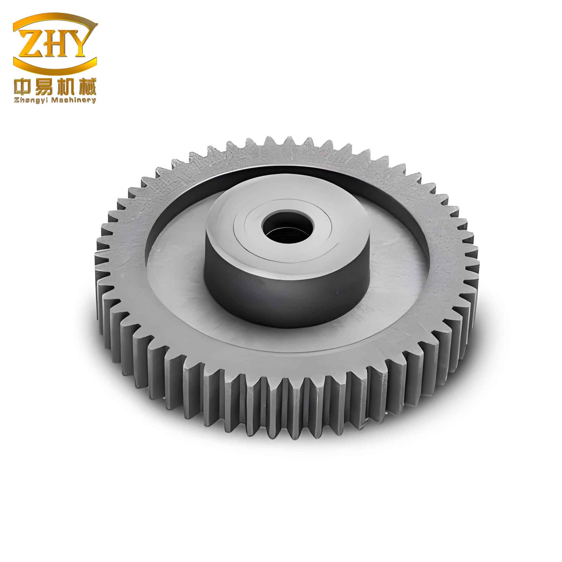
The system architecture is designed as a sequential pipeline. It begins with the acquisition and preprocessing of the spur and pinion gear image to enhance quality and segment the gear from the background. Subsequently, a dimensional metrology step is performed on this image to obtain fundamental gear parameters. These parameters are then used to generate a precise, pixel-level model of the standard involute tooth profile for each tooth. Concurrently, the actual contour of every tooth on the spur and pinion gear is extracted from the processed image. Finally, for each tooth position, a metric quantifying the shape difference between the actual and ideal contours is calculated. The evaluation of this metric against a predefined tolerance threshold forms the basis for the pass/fail decision on each tooth, completing the defect detection cycle for the spur and pinion gear.
Image Acquisition, Preprocessing, and Segmentation
The implementation leverages the HALCON machine vision library, utilizing its extensive set of optimized operators. The development workflow involves prototyping algorithms in HALCON’s interactive HDevelop environment and subsequently exporting them as C++ code for integration into a final application framework, such as one built with Microsoft Visual Studio. This combines algorithmic power with a custom user interface.
For image capture, I use an industrial camera (e.g., MV-EM 120C) with a resolution of 1280 x 960 pixels. The system is calibrated to achieve a known measurement precision, for instance, 0.05 mm per pixel. The image acquisition is initiated using HALCON operators like `grab_image_start`.
Acquired images are invariably contaminated by noise, such as salt-and-pepper and Gaussian noise, which can interfere with subsequent analysis. A two-stage filtering process is applied. First, a median filter (`median_image`) effectively removes salt-and-pepper noise. This is followed by a Gaussian filter (`gauss_image`) to smooth out Gaussian noise, resulting in a cleaner image suitable for precise edge detection.
The next critical step is image segmentation, isolating the spur and pinion gear (foreground) from the background. This is achieved through global thresholding. By analyzing the image’s grayscale histogram, a suitable threshold value \( M \) is selected. The binarization operation is defined as:
$$ g(x,y) = \begin{cases} 1 & \text{if } f(x,y) < M \\ 0 & \text{if } f(x,y) \ge M \end{cases} $$
where \( f(x,y) \) is the original grayscale image and \( g(x,y) \) is the resulting binary image, with 1 typically representing the object (the spur and pinion gear) and 0 the background. The HALCON operator `threshold(Image, Regions, MinGray, MaxGray)` performs this operation, where pixels with gray values within `[MinGray, MaxGray]` are grouped into the object region.
Extracting Fundamental Parameters of the Spur and Pinion Gear
The binary image may contain small, disconnected noise regions alongside the main spur and pinion gear region. The `connection` operator separates all connected components. Since the gear is typically the largest object in the field of view, the `select_shape_std` operator is used to select the region with the ‘max_area’, effectively isolating the spur and pinion gear for measurement.
Key geometric parameters are extracted directly from this segmented region. First, internal holes (e.g., the bore) are filled using `fill_up` to avoid interference. The smallest enclosing circle (`smallest_circle`) gives the center coordinates and the radius \( r_a \) of the tip circle. The largest inscribed circle (`inner_circle`) provides the center and radius \( r_f \) of the root circle. The tip and root diameters are then \( d_a = 2r_a \) and \( d_f = 2r_f \), respectively.
Determining the number of teeth \( Z \) is crucial. A circular region matching the root circle is generated (`gen_circle`), and its complement is obtained (`complement`). The intersection (`intersection`) of this complement region with the original filled gear region yields a region containing only the teeth. Applying the `connection` operator to this result separates individual teeth, and `count_obj` gives the total tooth count \( Z \). With \( Z \) and \( d_a \), the module \( m \) (for standard spur and pinion gears with no profile shift) can be approximated as \( m \approx d_a / (Z + 2) \). The pitch diameter \( d \) is \( d = m \cdot Z \). Assuming a standard pressure angle \( \alpha \) (commonly 20°), the base circle diameter \( d_b \) is calculated as \( d_b = d \cdot \cos(\alpha) \). The angular pitch \( P \) is \( P = 360^\circ / Z \).
| Parameter | Symbol | Extraction Method / Formula |
|---|---|---|
| Tip Diameter | \( d_a \) | `smallest_circle` → \( d_a = 2 \times \text{OuterRadius} \) |
| Root Diameter | \( d_f \) | `inner_circle` → \( d_f = 2 \times \text{InnerRadius} \) |
| Number of Teeth | \( Z \) | Tooth region isolation & `count_obj` |
| Module | \( m \) | \( m \approx d_a / (Z + 2) \) |
| Pitch Diameter | \( d \) | \( d = m \cdot Z \) |
| Base Diameter | \( d_b \) | \( d_b = d \cdot \cos(\alpha) \) |
| Angular Pitch | \( P \) | \( P = 360^\circ / Z \) |
Generation of the Standard Involute Tooth Profile
The standard contour for a spur and pinion gear tooth is an involute curve bounded by the tip and root circles. The involute of a circle can be parametrically generated. Let \( r_b \) be the base circle radius. For a rolling angle \( \gamma \) (in radians), the length of the unwound tangent (the generating line) is \( s = \gamma \cdot r_b \). The coordinates of a point on the involute are given by:
$$ \begin{aligned} x_1 &= r_b \cdot \cos(\gamma) \\ y_1 &= r_b \cdot \sin(\gamma) \\ x &= x_1 + s \cdot \sin(\gamma) = r_b (\cos(\gamma) + \gamma \sin(\gamma)) \\ y &= y_1 – s \cdot \cos(\gamma) = r_b (\sin(\gamma) – \gamma \cos(\gamma)) \end{aligned} $$
Using these equations with \( \gamma \) ranging from 0 to a value where the radius reaches the tip circle radius, the involute curve is discretized. Two such curves are generated, mirrored to form the left and right flanks of a tooth centered on the horizontal axis. These curve segments are trimmed at their intersections with the tip circle and root circle (or fillet limit). This yields a closed, sub-pixel accurate contour representing one perfect tooth of the spur and pinion gear. By rotating this master contour around the gear center by multiples of the angular pitch \( P \), the complete set of reference tooth profiles for the entire spur and pinion gear is generated.
Extraction of Actual Tooth Contours
To compare the actual spur and pinion gear against the standard model, the contour of each physical tooth must be extracted. First, the gear image needs to be aligned so that a reference tooth is in a known orientation (e.g., upright). A single tooth contour is extracted initially. The intersections of this contour with the base circle are computed. The line connecting the midpoint of these two intersection points to the gear center defines the tooth’s central axis. The angle \( \beta \) between this axis and the horizontal is calculated. The entire gear image is then rotated by \( -\beta \) degrees, aligning that specific tooth symmetrically. After rotation, the image is re-binarized and segmented. Each individual tooth region is isolated using `connection`. The `gen_contour_region_xld` operator with the ‘border’ option extracts a sub-pixel precise polygonal contour for each tooth region, resulting in a set of actual contour points \( A_i \) for tooth \( i \).
Core Detection Algorithm: The Hausdorff Distance
The Hausdorff distance is a robust metric for quantifying the dissimilarity between two sets of points or curves. It is particularly effective for shape comparison in tasks like image matching and defect detection. For two planar curves \( A \) and \( B \), the one-way (directed) Hausdorff distance from \( A \) to \( B \) is defined as:
$$ h(A, B) = \max_{a \in A} \left( \min_{b \in B} d(a, b) \right) $$
where \( d(a, b) \) is the Euclidean distance between points \( a \) and \( b \). In essence, for every point on curve \( A \), we find the distance to the closest point on curve \( B \), and then take the maximum of these minimum distances. It represents the maximum distance from curve \( A \) to curve \( B \). Similarly, the directed distance from \( B \) to \( A \) is:
$$ h(B, A) = \max_{b \in B} \left( \min_{a \in A} d(b, a) \right) $$
The (two-way) Hausdorff distance, which is symmetric and used as the overall measure of deviation, is the maximum of the two directed distances:
$$ H(A, B) = \max \left( h(A, B), h(B, A) \right) $$
This metric \( H \) tells us the maximum possible distance one would need to move any point on one contour to match the other contour, making it sensitive to localized gross deviations like a chip or wear scar on a spur and pinion gear tooth.
Defect Detection Methodology for Spur and Pinion Gears
For each tooth \( i \) on the spur and pinion gear, I compute the Hausdorff distance \( H_i \) between its extracted actual contour \( A_i \) and the corresponding generated standard contour \( S_i \). The tooth is flagged as defective if \( H_i \) exceeds a predefined tolerance threshold \( E \).
The total permissible tolerance \( E \) is composed of several factors: the allowable manufacturing tolerance (gear quality grade), systematic errors from imaging, and algorithmic errors. According to gear handbooks, the total profile deviation \( F_\alpha \) is the permissible range between two theoretically ideal profiles. The actual profile trace must lie within this band. Therefore, half of this value, \( F_\alpha / 2 \), is used as the geometric tolerance. Imaging factors (lighting, slight blur) and edge extraction inaccuracies contribute an estimated error of about 1 pixel. The alignment rotation step, based on pixel coordinates, introduces a further minor error, estimated at 0.5 pixels. Thus, the composite detection threshold is:
$$ E = \frac{F_\alpha}{2} + 1.0 + 0.5 \text{ (in pixels)} $$
The value of \( F_\alpha \) in pixels is derived from the gear’s quality grade (e.g., ISO 1328 Grade 12) and module, divided by the pixel calibration factor (e.g., 0.05 mm/pixel).
The algorithmic workflow in the final application follows these steps sequentially: Image Acquisition → Preprocessing → Parameter Extraction → Standard Profile Generation → Image Rotation → Actual Contour Extraction → Hausdorff Distance Calculation → Defect Classification. Teeth classified as defective are visually highlighted in the results.
Application Case Studies
Case 1: Detection of a Broken Tooth on a Spur and Pinion Gear
A spur and pinion gear with 18 teeth and one fractured tooth was inspected. System measurements yielded: \( Z=18 \), \( m \approx 2.4996 \), \( d \approx 44.9928 \) mm. For a grade 12 gear of this module, the handbook value for \( F_\alpha \) is approximately 81 µm. With a calibration of 0.05 mm/pixel, \( F_\alpha \approx 1.62 \) pixels. The total tolerance is calculated as \( E = 0.81 + 1.0 + 0.5 = 2.31 \) pixels. The Hausdorff distances for all 18 teeth were computed.
| Tooth Index | Hausdorff Distance \( H_i \) (pixels) | Judgment (E=2.31) |
|---|---|---|
| 0 | 1.6877 | OK |
| 1 | 1.9161 | OK |
| 2 | 7.3483 | DEFECT |
| 3 | 2.0789 | OK |
| 4 | 1.8528 | OK |
| … | … | … |
| 17 | 1.3309 | OK |
The algorithm successfully identified tooth #2 as defective due to its significantly higher Hausdorff distance (7.35 > 2.31), corresponding precisely to the broken tooth on the spur and pinion gear. Other teeth show distances within the acceptable tolerance band.
Case 2: Detection of Wear on a Used Spur and Pinion Gear
A worn spur and pinion gear with 16 teeth was analyzed. Measured parameters: \( Z=16 \), \( m \approx 1.9893 \), \( d \approx 31.8288 \) mm. The corresponding \( F_\alpha \) for grade 12 is about 58 µm, or 1.16 pixels. The total tolerance is \( E = 0.58 + 1.0 + 0.5 = 2.08 \) pixels.
| Tooth Index | Hausdorff Distance \( H_i \) (pixels) | Judgment (E=2.08) |
|---|---|---|
| 0 | 2.9154 | DEFECT |
| 1 | 2.1121 | OK (Marginal) |
| 2 | 2.1973 | DEFECT |
| 3 | 2.7148 | DEFECT |
| 4 | 1.8988 | OK |
| … | … | … |
| 15 | 3.0096 | DEFECT |
In this case, over half of the teeth on the spur and pinion gear exhibited Hausdorff distances exceeding the 2.08-pixel threshold, correctly identifying them as worn or damaged. This demonstrates the method’s effectiveness in assessing the condition of used spur and pinion gears for potential reusability.
Conclusion
I have presented a complete, automated vision-based inspection system for detecting tooth profile defects in standard involute spur and pinion gears. The methodology integrates robust image processing for gear isolation and parameter extraction, precise geometric modeling for generating ideal involute profiles, and a contour comparison based on the Hausdorff distance metric. The system’s effectiveness is validated through successful detection of both catastrophic failures (tooth breakage) and progressive wear in spur and pinion gears. By comparing the manufactured or worn profile against a mathematically perfect standard, this approach provides an objective, quantitative, and non-contact assessment. The technique is well-suited for inline quality control in manufacturing lines for spur and pinion gears and for condition monitoring of gears in service. The modular design of the algorithm pipeline allows for adaptation to inspect other types of gears by modifying the profile generation model accordingly, highlighting its versatility in industrial machine vision applications.