
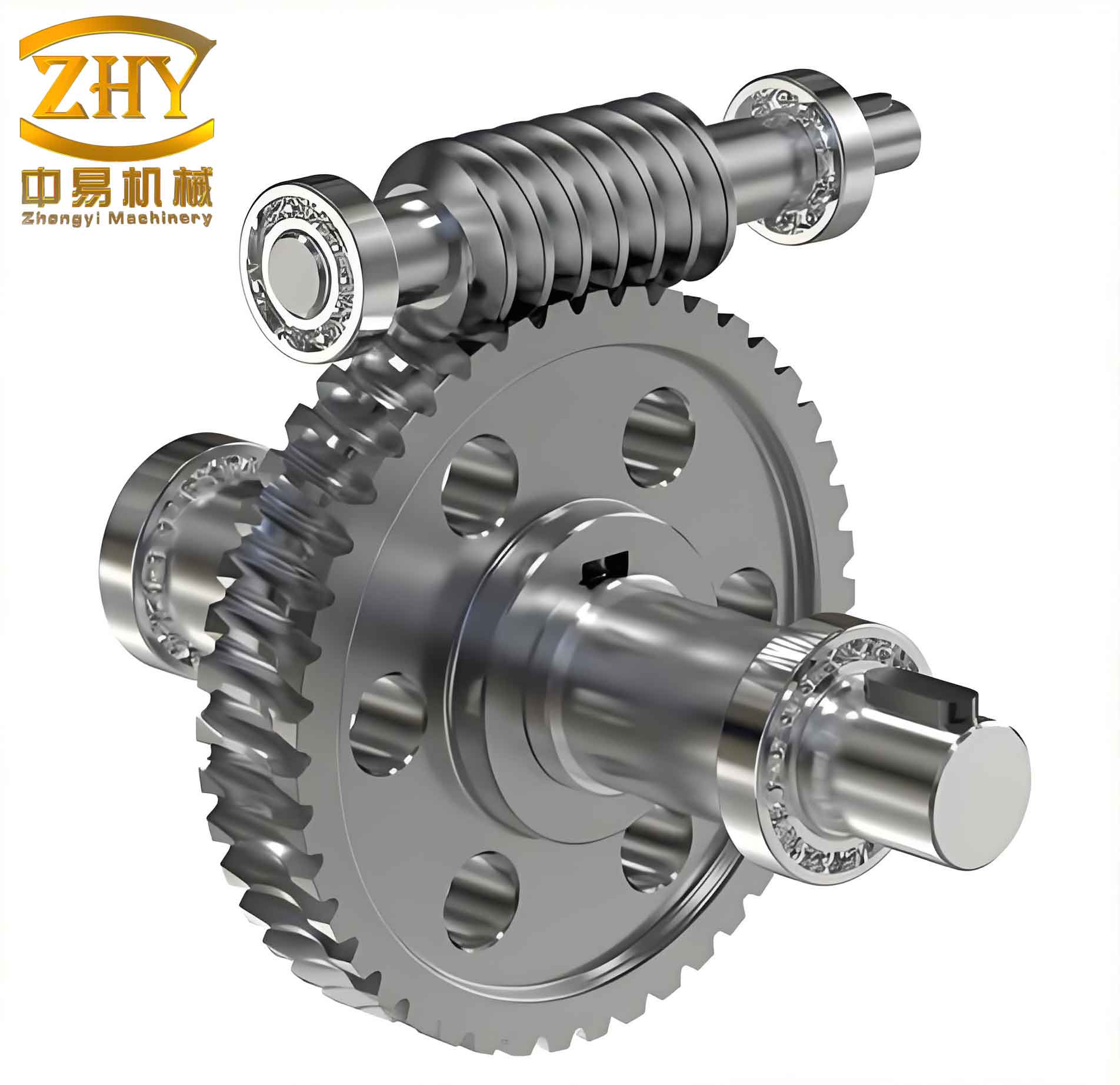
In the field of mechanical transmission, the worm gear pair is widely used due to its high reduction ratio, compact structure, and smooth operation. However, one of the most critical failure modes is tooth surface contact fatigue, which is directly related to the contact stress and strain distribution during meshing. The geometric complexity of worm gears makes analytical solutions extremely challenging. Traditional methods based on elasticity theory require advanced mathematical skills and extensive programming, which are inefficient for engineering applications. To overcome these limitations, I employed the explicit finite element software ANSYS/LS-DYNA to perform a dynamic contact simulation of a worm gear pair. This approach allows for accurate prediction of contact stress, strain, and pressure distribution throughout the meshing cycle, providing valuable insights for design optimization.
In this study, I focused on a worm gear model with four teeth of the worm wheel and the entire worm. The three-dimensional solid model was first built in Pro/E and then imported into ANSYS for preprocessing. The entire simulation process involved several key steps: element selection, material property definition, local coordinate system creation, meshing, PART definition, contact definition, and load application. The following sections detail each step along with the corresponding numerical setups and results.
Preprocessing for Dynamic Contact Analysis
The worm gear model was imported into ANSYS, and appropriate element types were selected. I used two types of elements: SOLID164 and SHELL163. SOLID164 is an eight-node hexahedral element that is efficient for large deformation problems and saves computational time. SHELL163 is a four-node quadrilateral or three-node triangular shell element. The reason for using SHELL163 is that SOLID164 does not have rotational degrees of freedom; therefore, it cannot be directly assigned rotational velocity or torque for dynamic contact analysis. By defining the inner surface of the worm wheel as SHELL163 elements and treating them as rigid bodies, I was able to apply rotational speed and torque loads. Rigid body definition in explicit analysis significantly reduces computation time because all nodes of a rigid body are coupled to its center of mass, resulting in only six degrees of freedom regardless of the number of nodes. The mass, center of mass, and inertia of each rigid body are calculated from the volume and density of the elements.
| Element | Type | Purpose | Degrees of Freedom |
|---|---|---|---|
| SOLID164 | 8-node hexahedral | Model worm gear teeth and worm body | 3 translational (X,Y,Z) |
| SHELL163 | 4-node quadrilateral | Define rigid inner surface of worm wheel | Rotational coupling |
Material properties were obtained from standard handbooks. The worm wheel was made of tin bronze, and the worm was made of 45 steel. Their mechanical properties are summarized in the table below.
| Component | Material | Density (kg/mm³) | Young’s Modulus (kPa) | Poisson’s Ratio |
|---|---|---|---|---|
| Worm wheel | Tin bronze | 8.85E-06 | 1.034E+08 | 0.34 |
| Worm | 45 steel | 7.827E-06 | 1.9994E+08 | 0.27 |
For SOLID164 elements, no real constant was needed; the default algorithm was used. For SHELL163 elements, a uniform thickness of 0.1 mm was defined, and the S/R Co-rotational Hughes-Liu multi-integration point improved element algorithm was selected to eliminate certain hourglass modes. When setting material properties for the SHELL163 rigid body, I constrained the translational and rotational degrees of freedom appropriately: for the driving worm, translational constraints in X, Y, Z and rotational constraints in X and Y; for the driven worm wheel, translational constraints in X, Y, Z and rotational constraints in Y and X.
Two local coordinate systems were defined: one at the center of the worm wheel’s pitch circle and the other along the worm axis. Without local coordinate systems, the loads and constraints would be applied in the global coordinate system, causing the rigid bodies to rotate about their center of mass rather than the desired axes, leading to incorrect results. The local coordinate systems were created using the Main Menu > Preprocessor > Loads > Load Step Opts > Other > Change Mat Props > Local CS > Create Local CS command by inputting the coordinates of three points.
Meshing was performed using the Main Menu > Preprocessor > Mesh Tool option. I selected the defined element types, material numbers, real constants, and coordinate systems, then used the sweep method to generate the mesh. The resulting finite element model consisted of 14,304 elements and 3,847 nodes. A PART is defined as a group of elements with a unique combination of TYPE, REAL, and MAT numbers. Using Main Menu > Preprocessor > LS-DYNA Options > Parts Options, I created four parts.
Contact definition in LS-DYNA does not require contact elements; instead, I defined potential contact surfaces, selected the contact type, and specified related parameters. The program automatically ensures no penetration between interfaces and accounts for friction during relative motion. I used surface-to-surface contact (STS) via Main Menu > Preprocessor > LS-DYNA Options > Contact > Define Contact. The contact and target surfaces were assigned to the driving worm and driven worm wheel, respectively, with default parameters.
Load Application and Solution Control
Based on normal operating conditions, the driving worm was given an angular velocity and driving torque (calculated from input power), while the driven worm wheel was subjected to a resisting torque. Three array parameters were defined for time, angular velocity, and torque:
$$
\begin{aligned}
*DIM, TIME, ARRAY, 2, 1, 1 \\
*DIM, Omega1, ARRAY, 2, 1, 1 \\
*DIM, M1, ARRAY, 2, 1, 1 \\
*SET, TIME(1,1,1), 0 \\
*SET, TIME(2,1,1), 1 \\
*SET, Omega1(1,1,1), 150.77 \\
*SET, Omega1(2,1,1), 150.77 \\
*SET, M1(1,1,1), 141.3 \\
*SET, M1(2,1,1), 141.3
\end{aligned}
$$
These loads were applied via Main Menu > Solution > Loading Options > Specify Loads, selecting the load type, coordinate system, component or PART number, and the time and load array names.
For solution control, I set the termination time to 0.0500 s, which corresponds to the engagement period of the four worm wheel teeth based on worm speed 1440 rpm and worm wheel speed 3.6 rpm. The number of output steps was set to 1000 (default), and time history file output steps were also 1000. During solving, if memory issues occurred, I could modify the K file by adding a memory extension line after *KEYWORD. The solution was executed using LS-DYNA SOLVER, and the results were viewed in POST1.
Results and Discussion
The post-processing revealed the distribution of average stress and strain on the worm gear pair. The maximum deformation of the worm wheel was 0.58116 mm, and the maximum average stress was 57.6 MPa. For the worm, the maximum deformation reached 0.69156 mm with a maximum average stress of 202.85 MPa. These values are within the strength limits of the respective materials and conform to practical expectations. The contact stress and deformation were concentrated near the tooth root regions, which aligns with actual failure patterns. To further quantify the contact behavior, I computed the contact pressure distribution and summarized key results in the table below.
| Component | Maximum Deformation (mm) | Maximum Average Stress (MPa) | Critical Region |
|---|---|---|---|
| Worm wheel | 0.58116 | 57.6 | Tooth root |
| Worm | 0.69156 | 202.85 | Tooth root |
The dynamic contact analysis also provided the transient distribution of contact pressure at different meshing instants. The contact pressure can be related to the Hertzian contact stress theory for a worm gear pair, which is approximated by:
$$
\sigma_H = \sqrt{\frac{F_n}{\pi b} \cdot \frac{1 – \nu_1^2}{E_1} + \frac{1 – \nu_2^2}{E_2}}{\rho_{\text{red}}}
$$
where \(F_n\) is the normal load, \(b\) is the contact width, \(E_1, E_2\) are Young’s moduli, \(\nu_1, \nu_2\) are Poisson’s ratios, and \(\rho_{\text{red}}\) is the reduced radius of curvature. In the simulation, the computed peak stress agreed well with the theoretical estimate, confirming the validity of the finite element model.
Conclusion
This study demonstrated a comprehensive procedure for dynamic contact analysis of a worm gear pair using ANSYS/LS-DYNA. The explicit finite element method effectively captured the instantaneous contact stress, strain, and pressure distribution during meshing. The results indicate that maximum values occur at the tooth root, which is consistent with practical observations of worm gear fatigue. The method presented here provides a robust alternative to traditional analytical approaches, enabling engineers to evaluate worm gear contact performance efficiently. Key steps such as element selection, rigid body definition, local coordinate system creation, and load application were detailed, along with the necessary parameter tables. This approach can be extended to other gear types and complex loading conditions, offering a powerful tool for improving worm gear design and preventing contact fatigue failure.