
Throughout my research on worm gear transmissions, I have been fascinated by the unique capabilities of straight toroidal worm gear drives. These drives, originally invented by Hindley and later refined by Cone and Lorenz, offer distinct advantages over enveloping worm gear drives, including better resistance to tooth tip thinning and simpler manufacturing of the hob. However, they suffer from limited conjugate contact area and the presence of constant contact lines on the worm gear tooth surface, which can lead to early failure. To overcome these drawbacks, various modification methods have been proposed. Among them, the natural modification method based on measured wear curves and the rational modification method based on gear meshing theory have been widely studied.
In my work, I systematically develop a mathematical model for high-order modified straight toroidal worm gear drives. Starting from the natural modification data, I first normalize the data to obtain a universal modification curve using high-order polynomial fitting. Then, I derive the relationship between this curve and the process transmission ratio, which governs the cutting motion during worm gear manufacturing. Using differential geometry and gear meshing theory, I compute the curvature parameters, meshing function, and curvature interference boundary function for the worm gear pair. I also prove that the worm gear tooth surface is a non-developable ruled surface, which aligns with the fundamental forming principle of the worm gear. Finally, I present numerical examples for different modification curves (cubic, quintic, and septic) and analyze their effects on contact patterns, conjugate areas, and local meshing characteristics.
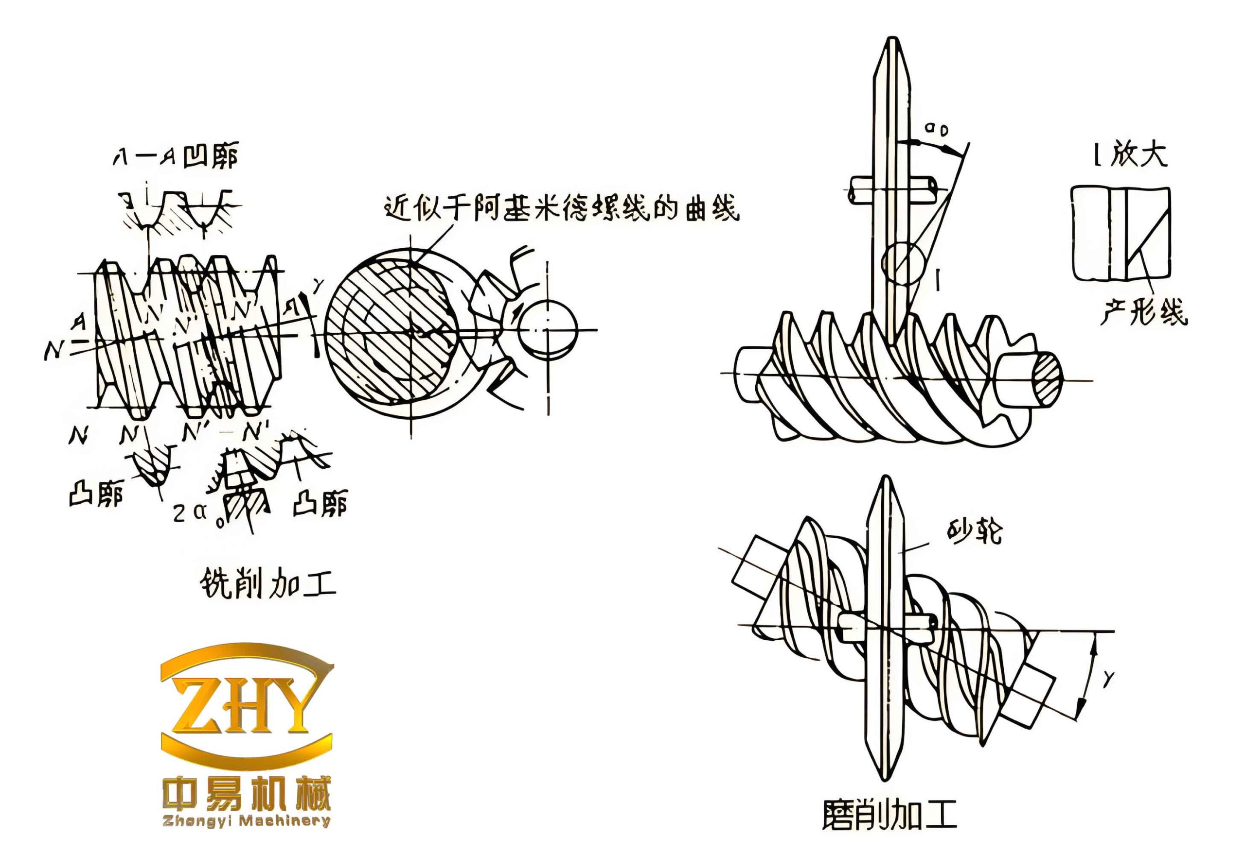
1. Mathematical Model for Worm Gear Tooth Surface
When I began the analysis, I first defined the cutting tool geometry. The straight-edged turning tool used to generate the worm gear tooth surface is described in the tool coordinate system by:
$$(\mathbf{r}_d)_d = -u\,\mathbf{i}_d + r_b\,\mathbf{j}_d$$
where \(u\) is the tool parameter, and \(r_b\) is the base radius. The tool is rotated about the worm gear axis by an angle \(\varphi_d\) during manufacturing. By applying rotational transformations, I obtained the worm gear tooth surface equation in the moving coordinate system \(\sigma_{od}\):
$$(\mathbf{r}_d)_{od} = \mathbf{R}[\mathbf{k}_{od},\varphi_d] (\mathbf{r}_d)_d = x_{od}\,\mathbf{i}_{od} + y_{od}\,\mathbf{j}_{od}$$
with
$$x_{od} = -u\cos\varphi_d – r_b\sin\varphi_d,\quad y_{od} = -u\sin\varphi_d + r_b\cos\varphi_d$$
Finally, in the worm gear fixed coordinate system \(\sigma_1\), the tooth surface is:
$$(\mathbf{r}_1)_1 = a\,\mathbf{R}[\mathbf{k}_1,-\varphi]\mathbf{i}_{o1} + \mathbf{R}[\mathbf{k}_1,-\varphi]\,\mathbf{R}\left[\mathbf{i}_{o1},\frac{\pi}{2}\right] (\mathbf{r}_d)_{od}$$
2. Proof of Non-Developability of the Worm Gear Tooth Surface
It is known that the worm gear tooth surface is a ruled surface, but its developability has not been rigorously proven. I wrote the surface as:
$$(\mathbf{r}_1)_1 = \boldsymbol{\rho}(\varphi) + u\,\mathbf{t}(\varphi)$$
Then I computed the derivatives with respect to \(\varphi\) and evaluated the scalar triple product:
$$[\boldsymbol{\rho}'(\varphi),\mathbf{t}(\varphi),\mathbf{t}'(\varphi)] = \frac{1}{i_{1d}}(a – r_b\sin\varphi_d) \neq 0$$
Since this value is never zero, the surface is non-developable, confirming the classical understanding that a straight toroidal worm gear tooth surface cannot be flattened onto a plane without distortion.
3. High-Order Modification Curve
To improve the fitting accuracy of the natural modification curve, I first normalized the experimental data from reference [9] using the following coefficients:
Rotation coefficient: \(x = \frac{\varphi_x}{\varphi_w} = \frac{i_{12}\alpha – \varphi}{i_{12}\varphi_w}\)
Modification coefficient: \(I_i = \frac{\Delta_{(i)s}}{\Delta_f}\)
where \(\Delta_f\) is the modification amount at the worm gear entrance, calculated by:
$$\Delta_f = a(0.0003 + 0.000034i_{12})$$
After processing 35 sets of data points, I used the least squares method to fit the following polynomial of degree \(n\):
$$I_n(x) = \sum_{k=0}^n c_k x^k$$
The coefficients for different polynomial degrees are summarized in Table 1.
| Coefficient | Cubic | 4th power | 5th power | 6th power | 7th power |
|---|---|---|---|---|---|
| \(c_0\) | 9.9857×10⁻² | 1.0202×10⁻¹ | 1.0202×10⁻¹ | 9.6396×10⁻² | 9.640×10⁻² |
| \(c_1\) | 5.0056×10⁻¹ | 5.0056×10⁻¹ | 5.2125×10⁻¹ | 5.2125×10⁻¹ | 5.1184×10⁻¹ |
| \(c_2\) | 4.2790×10⁻¹ | 4.0739×10⁻¹ | 4.0739×10⁻¹ | 5.2004×10⁻¹ | 5.2004×10⁻¹ |
| \(c_3\) | -4.5089×10⁻² | -4.5089×10⁻² | -1.3687×10⁻¹ | -1.3687×10⁻¹ | -5.5751×10⁻² |
| \(c_4\) | 0 | -2.2659×10⁻² | -2.2659×10⁻² | -2.9935×10⁻¹ | -2.9935×10⁻¹ |
| \(c_5\) | 0 | 0 | 7.8395×10⁻² | 7.8395×10⁻² | -9.2200×10⁻² |
| \(c_6\) | 0 | 0 | 0 | 2.2474×10⁻¹ | 2.2474×10⁻¹ |
| \(c_7\) | 0 | 0 | 0 | 0 | 1.0084×10⁻¹ |
The total fitting errors (sum of squared residuals) for each polynomial degree are shown in Table 2.
| Polynomial degree | 2 | 3 | 4 | 5 | 6 | 7 |
|---|---|---|---|---|---|---|
| Error | 6.9852×10⁻² | 5.4385×10⁻² | 5.3239×10⁻² | 4.9359×10⁻² | 3.9980×10⁻² | 3.9457×10⁻² |
The results indicate that simply increasing the polynomial degree does not dramatically improve accuracy. The modification amount function is then used to derive the process transmission ratio:
$$i_{1d} = \frac{i_{12}}{1 + \frac{\Delta_f}{r_2 \varphi_w} I’_n(x)}$$
where \(I’_n(x) = \sum_{k=1}^n k c_k x^{k-1}\).
4. Meshing Theory for High-Order Modified Worm Gear
I established a coordinate system consisting of six frames: three moving frames attached to the worm gear, worm wheel, and tool, and three fixed frames. Using the tool geometry and process transmission ratio, I derived the worm gear tooth surface equation and its fundamental quantities.
The first fundamental form coefficients are:
$$E = 1,\quad F = \frac{r_b}{i_{1d}},\quad G = (x_{od}+a)^2 + \left(u^2 + \frac{r_b^2}{i_{1d}^2}\right)$$
The unit normal vector to the worm gear tooth surface is:
$$(\mathbf{n}_1)_1 = \frac{1}{D} \mathbf{R}[\mathbf{k}_1,-\varphi] \mathbf{R}\left[\mathbf{i}_{o1},\frac{\pi}{2}\right] \mathbf{R}[\mathbf{k}_{od},\varphi_d] \left[(a+x_{od})\mathbf{j}_d + \frac{u}{i_{1d}}\mathbf{k}_d\right]$$
where \(D = \sqrt{(u/i_{1d})^2 + (a+x_{od})^2}\).
The second fundamental form coefficients are:
$$L = 0,\quad M = \frac{r_b\sin\varphi_d – a}{i_{1d} D},\quad N = \frac{a+x_{od}}{D} \left[(a+x_{od})\sin\varphi_d – u\frac{d^2\varphi_d}{d\varphi^2} – \frac{r_b}{i_{1d}^2}\right] – \frac{2u y_{od}}{i_{1d}^2 D}$$
From these, I obtained the normal curvature along the direction \(\boldsymbol{\alpha}_\xi\):
$$k_\xi = \frac{L}{E} = 0$$
and the geodesic torsion:
$$\tau_\xi = \frac{M}{D}$$
The meshing function for the worm gear pair is:
$$\Phi(u,\varphi,\varphi_1) = (\mathbf{n}_1^*)_{o1} \cdot (\mathbf{V}_{12})_{o1} = \frac{1}{i_{12} D} [A\sin(\varphi_1-\varphi) + B\cos(\varphi_1-\varphi) + C]$$
with:
$$A = \frac{u y_{od}}{i_{1d}},\quad B = (x_{od}+a)(u – a\cos\varphi_d),\quad C = (x_{od}+a)\left(a\cos\varphi_d – \frac{i_{12}}{i_{1d}} u\right)$$
Setting \(\Phi = 0\) gives the condition for meshing contact.
5. Curvature Interference and Local Meshing Characteristics
The curvature interference boundary function is:
$$\Psi = N_\xi (\mathbf{V}_{12})_{o1}\cdot \boldsymbol{\alpha}_\xi + N_\eta (\mathbf{V}_{12})_{o1}\cdot \boldsymbol{\alpha}_\eta + \Phi_{\varphi_1}$$
where
$$\Phi_{\varphi_1} = \frac{1}{i_{12} D}[A\cos(\varphi_1-\varphi) – B\sin(\varphi_1-\varphi)]$$
The components \(N_\xi\) and \(N_\eta\) are functions of the surface curvatures and relative motion. The induced normal curvature along the contact line is:
$$k_N^{(12)} = \frac{N_\xi^2 + N_\eta^2}{\Psi}$$
and the sliding angle:
$$\theta_{vt} = \arcsin\left|\frac{\Psi – \Phi_{\varphi_1}}{|\mathbf{V}_{12}|_{o1} \sqrt{N_\xi^2 + N_\eta^2}}\right|$$
6. Numerical Examples and Analysis
I applied the theoretical model to a specific worm gear pair with parameters: number of worm gear starts \(Z_1 = 2\), center distance \(a = 280\) mm, transmission ratio \(i_{12} = 25\). The complete design parameters are listed in Table 3.
| Parameter | Value |
|---|---|
| Worm gear pitch diameter (mm) | 94 |
| Worm wheel pitch diameter (mm) | 466 |
| Face width of worm wheel (mm) | 70 |
| Base circle diameter (mm) | 175 |
| Pressure angle (°) | 22.0589 |
| Number of worm wheel teeth | 50 |
| Transverse module (mm) | 9.32 |
| Number of worm gear enveloping teeth | 5 |
| Working half-angle of worm gear (°) | 16.3809 |
| Working length of worm gear (mm) | 131.42 |
| Addendum circle diameter of worm gear (mm) | 107.98 |
| Addendum circle diameter of worm wheel (mm) | 479.98 |
| Maximum addendum circle diameter of worm wheel (mm) | 489 |
| Addendum arc radius of worm gear (mm) | 226.01 |
| Addendum arc radius of worm wheel (mm) | 41 |
| Root arc radius of worm wheel (mm) | 55.854 |
| Entrance modification amount (mm) | 0.3239 |
For the unmodified (primitive) worm gear drive, the conjugate region on the worm wheel tooth surface degenerates into a constant contact line, as shown by the meshing analysis. The only effective contact area is the secondary conjugate region \(\Sigma_B\), which is bounded by a curvature interference line. The induced normal curvature and sliding angle in \(\Sigma_B\) are favorable, but the region is limited to the exit side of the worm gear.
When I applied high-order modification (cubic, quintic, and septic curves), the constant contact line disappeared, and both conjugate regions \(\Sigma_A\) and \(\Sigma_B\) expanded significantly. Tables 4–6 present the computed local meshing parameters for three modification cases.
| Contact line | Point a | Point b | Point c | |||
|---|---|---|---|---|---|---|
| \(k_N^{(12)}\) (mm⁻¹) | \(\theta_{vt}\) (°) | \(k_N^{(12)}\) (mm⁻¹) | \(\theta_{vt}\) (°) | \(k_N^{(12)}\) (mm⁻¹) | \(\theta_{vt}\) (°) | |
| 1 (first contact line) | 0.1170 | 83.46 | 0.0747 | 84.67 | 0.0498 | 85.79 |
| 1′ | 0.0076 | 50.98 | 0.0066 | 56.10 | 0.0059 | 61.40 |
| 2′ | 0.0056 | 61.67 | 0.0052 | 66.73 | 0.0050 | 70.33 |
| 3′ | 0.0026 | 83.95 | 0.0027 | 83.06 | 0.0028 | 82.63 |
| 4′ | 0.0069 | 86.49 | 0.0033 | 87.42 | 0.0018 | 88.20 |
| 5′ | 0.0155 | 83.15 | 0.0086 | 82.41 | 0.0047 | 80.61 |
| Contact line | Point a | Point b | Point c | |||
|---|---|---|---|---|---|---|
| \(k_N^{(12)}\) (mm⁻¹) | \(\theta_{vt}\) (°) | \(k_N^{(12)}\) (mm⁻¹) | \(\theta_{vt}\) (°) | \(k_N^{(12)}\) (mm⁻¹) | \(\theta_{vt}\) (°) | |
| 1 | 0.0388 | 83.47 | 0.0264 | 84.73 | 0.0191 | 85.88 |
| 1′ | 0.0066 | 51.51 | 0.0056 | 56.33 | 0.0048 | 61.53 |
| 2′ | 0.0055 | 61.70 | 0.0051 | 66.78 | 0.0049 | 70.38 |
| 3′ | 0.0027 | 83.85 | 0.0028 | 82.96 | 0.0029 | 82.54 |
| 4′ | 0.0063 | 86.39 | 0.0030 | 87.30 | 0.0016 | 88.08 |
| 5′ | 0.0339 | 83.43 | 0.0212 | 82.83 | 0.0140 | 81.34 |
| Contact line | Point a | Point b | Point c | |||
|---|---|---|---|---|---|---|
| \(k_N^{(12)}\) (mm⁻¹) | \(\theta_{vt}\) (°) | \(k_N^{(12)}\) (mm⁻¹) | \(\theta_{vt}\) (°) | \(k_N^{(12)}\) (mm⁻¹) | \(\theta_{vt}\) (°) | |
| 1 | 0.0144 | 83.42 | 0.0102 | 84.67 | 0.0077 | 85.81 |
| 1′ | 0.0047 | 55.29 | 0.0039 | 59.47 | 0.0031 | 64.38 |
| 2′ | 0.0060 | 63.22 | 0.0057 | 68.29 | 0.0057 | 71.90 |
| 3′ | 0.0025 | 83.83 | 0.0026 | 83.32 | 0.0026 | 83.09 |
| 4′ | 0.0079 | 77.89 | 0.0038 | 81.63 | 0.0020 | 84.07 |
| 5′ | 0.0092 | 78.72 | 0.0049 | 70.97 | 0.0025 | 73.12 |
The results show that high-order modification effectively eliminates the constant contact line and increases the conjugate area. In the primitive drive, the only effective contact region \(\Sigma_B\) is limited to the exit side; after modification, both the entrance and exit sides participate in meshing, and the worm gear can be fully utilized along its entire length. The induced normal curvature remains small in both \(\Sigma_A\) and \(\Sigma_B\), indicating low contact stresses, and the sliding angle remains high, favoring oil film formation. However, a curvature interference line still exists in \(\Sigma_A\) for all modified cases, potentially leading to undercutting if the line crosses into the working tooth surface. With the septic modification, the curvature interference line is partially cut off by the exit boundary, reducing its harmful effect but not eliminating it completely.
7. Conclusions
From my comprehensive study, I draw the following conclusions:
- The high-order modification curve, derived from normalized natural wear data using polynomial fitting, provides a practical method to improve the meshing performance of straight toroidal worm gear drives. However, increasing the polynomial degree beyond three yields only marginal improvements in fitting accuracy.
- The mathematical model I developed, which incorporates the process transmission ratio as a variable rather than a constant, correctly accounts for the effect of modification on the entire meshing process. The proof of non-developability of the worm gear tooth surface confirms the fundamental geometric nature of these drives.
- Numerical examples demonstrate that high-order modification eliminates the constant contact line and significantly expands the conjugate area, allowing the worm gear to be used over its full length. The local meshing quality, measured by induced normal curvature and sliding angle, remains favorable.
- The main drawback is the presence of a curvature interference line in the primary conjugate region. While higher-order modifications can reduce the extent of this line, they cannot fully remove it. This suggests that high-order modification alone is not sufficient for optimal performance; it should be combined with other rational modification techniques to completely eliminate curvature interference.
In summary, the high-order modification principle offers a valuable tool for enhancing straight toroidal worm gear drives, but its limitations must be addressed through hybrid modification strategies. Future work will focus on integrating this method with other parameters such as center distance adjustment and tool axis inclination to achieve superior meshing performance.