
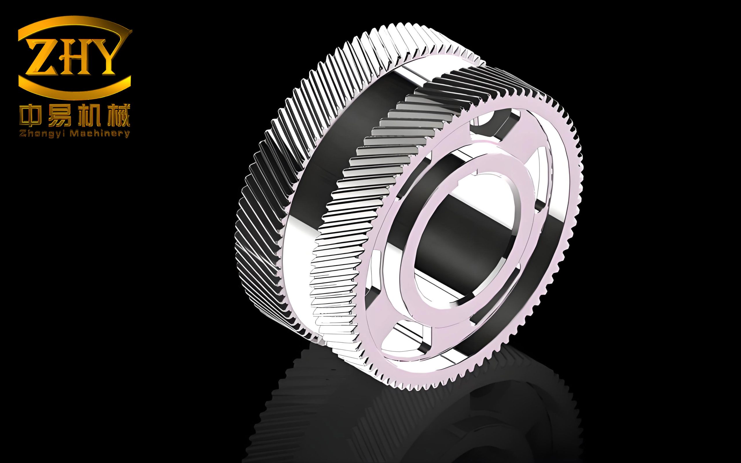
In my research, I have focused on the dynamic characteristics of high-speed herringbone gear transmission systems. Herringbone gears, formed by merging two helical gears with opposite helix directions, offer significant advantages in terms of smooth meshing, high torque transmission stability, and high load capacity. The axial forces generated by the two helical gear halves theoretically cancel each other, greatly reducing the load on thrust bearings. Therefore, herringbone gear systems are widely used in industries such as mining, chemical engineering, aviation, and heavy machinery.
Based on the finite element numerical analysis method, I derived the dynamic equations of the herringbone gear transmission system and established a rotor-bearing-gear dynamic system model. In the modeling process, I considered the effects of shear, bending, torsion, axial force, gyroscopic effect, and internal damping of the rotor shaft, as well as the time-varying mesh stiffness and transmission error of the herringbone gear pair. I also performed dynamic analysis on the high-speed gear rotor, and the results were in good agreement with the measured data from the test gearbox.
1. Dynamic Matrix Formulation
1.1 Dynamic Matrix of Flexible Shaft Segment
I primarily considered the dynamic characteristics of a flexible axisymmetric Euler shaft with shear, bending, torsion, axial force, gyroscopic effect, and internal damping. The rotor shaft was divided into several shaft segments. Each shaft segment element adopted a two-node, 8-degree-of-freedom Euler shaft element model, as shown in the finite element representation. Considering the degrees of freedom in the local coordinate system x-z and y-z planes, the generalized displacement vector is:
$$ \mathbf{q} = [u_1\; v_1\; \theta_1\; \psi_1\; u_2\; v_2\; \theta_2\; \psi_2]^T $$
The dynamic matrices are 8×8. Using the energy method, the dynamic matrices are obtained as follows:
(1) Stiffness Matrix of Shaft Element
$$ \mathbf{K}_s = \mathbf{K}_{se} + \mathbf{K}_{sFe} + \mathbf{K}_{sTe} + \mathbf{K}_{sce} $$
Where:
$$ \mathbf{K}_{se} = \frac{E_e I_e}{(1 + \Phi_e) l_e^3} \begin{bmatrix}
12 & 0 & 0 & 6l_e & -12 & 0 & 0 & 6l_e\\
0 & 12 & -6l_e & 0 & 0 & -12 & -6l_e & 0\\
0 & -6l_e & (4 + \Phi_e)l_e^2 & 0 & 0 & 6l_e & (2 – \Phi_e)l_e^2 & 0\\
6l_e & 0 & 0 & (4 + \Phi_e)l_e^2 & -6l_e & 0 & 0 & (2 – \Phi_e)l_e^2\\
-12 & 0 & 0 & -6l_e & 12 & 0 & 0 & -6l_e\\
0 & -12 & 6l_e & 0 & 0 & 12 & 6l_e & 0\\
0 & -6l_e & (2 – \Phi_e)l_e^2 & 0 & 0 & 6l_e & (4 + \Phi_e)l_e^2 & 0\\
6l_e & 0 & 0 & (2 – \Phi_e)l_e^2 & -6l_e & 0 & 0 & (4 + \Phi_e)l_e^2
\end{bmatrix} $$
$$ \mathbf{K}_{sFe} = \frac{f_e}{60(1 + \Phi_e)l_e} \begin{bmatrix}
k_1 & 0 & 0 & 6l_e & -k_1 & 0 & 0 & 6l_e\\
0 & k_1 & -6l_e & 0 & 0 & -k_1 & -6l_e & 0\\
0 & -6l_e & k_2 & 0 & 0 & 6l_e & k_3 & 0\\
6l_e & 0 & 0 & k_2 & -6l_e & 0 & 0 & k_3\\
-k_1 & 0 & 0 & -6l_e & k_1 & 0 & 0 & -6l_e\\
0 & -k_1 & 6l_e & 0 & 0 & k_1 & 6l_e & 0\\
0 & -6l_e & k_3 & 0 & 0 & 6l_e & k_2 & 0\\
6l_e & 0 & 0 & k_3 & -6l_e & 0 & 0 & k_2
\end{bmatrix} $$
$$ \mathbf{K}_{sTe} = \frac{t_e}{2l_e} \begin{bmatrix}
0 & 0 & 2 & 0 & 0 & 0 & -2 & 0\\
0 & 0 & 0 & 2 & 0 & 0 & 0 & -2\\
2 & 0 & 0 & -l_e & -2 & 0 & 0 & l_e\\
0 & 2 & l_e & 0 & 0 & -2 & -l_e & 0\\
0 & 0 & -2 & 0 & 0 & 0 & 2 & 0\\
0 & 0 & 0 & -2 & 0 & 0 & 0 & 2\\
-2 & 0 & 0 & -l_e & 2 & 0 & 0 & l_e\\
0 & -2 & l_e & 0 & 0 & 2 & -l_e & 0
\end{bmatrix} $$
$$ \mathbf{K}_{sce} = \frac{E_e I_e}{(1 + \Phi_e) l_e^3} \begin{bmatrix}
0 & 12 & -6l_e & 0 & 0 & -12 & -6l_e & 0\\
-12 & 0 & 0 & -6l_e & 12 & 0 & 0 & -6l_e\\
6l_e & 0 & 0 & (4 + \Phi_e)l_e^2 & -6l_e & 0 & 0 & (2 – \Phi_e)l_e^2\\
0 & 6l_e & -(4 + \Phi_e)l_e^2 & 0 & 0 & -6l_e & -(2 – \Phi_e)l_e^2 & 0\\
0 & -12 & 6l_e & 0 & 0 & 12 & 6l_e & 0\\
12 & 0 & 0 & 6l_e & -12 & 0 & 0 & 6l_e\\
6l_e & 0 & 0 & (2 – \Phi_e)l_e^2 & -6l_e & 0 & 0 & (4 + \Phi_e)l_e^2\\
0 & 6l_e & -(2 – \Phi_e)l_e^2 & 0 & 0 & -6l_e & -(4 + \Phi_e)l_e^2 & 0
\end{bmatrix} $$
Where:
$$ k_1 = 72 + 120\Phi_e + 60\Phi_e^2 $$
$$ k_2 = (8 + 10\Phi_e + 5\Phi_e^2) l_e^2 $$
$$ k_3 = -(2 + 10\Phi_e + 5\Phi_e^2) l_e^2 $$
$$ \Phi_e = \frac{12 E_e I_e}{k_e G_e A_e l_e^2} $$
$$ I_e = \frac{\pi r^4}{4}, \quad G_e = \frac{E_e}{2(1 + \nu)}, \quad k_e = \frac{6(1 + \nu)^2}{7 + 12\nu + 4\nu^2} $$
(2) Mass Matrix of Shaft Element
$$ \mathbf{M}_{se} = \frac{\rho_e A_e l_e}{840(1 + \Phi_e)^2} \begin{bmatrix}
m_1 & 0 & 0 & m_2 & m_3 & 0 & 0 & m_4\\
0 & m_1 & -m_2 & 0 & 0 & m_3 & -m_4 & 0\\
0 & -m_2 & m_5 & 0 & 0 & m_4 & m_6 & 0\\
m_2 & 0 & 0 & m_5 & -m_4 & 0 & 0 & m_6\\
m_3 & 0 & 0 & -m_4 & m_1 & 0 & 0 & -m_2\\
0 & m_3 & m_4 & 0 & 0 & m_1 & m_2 & 0\\
0 & -m_4 & m_6 & 0 & 0 & m_2 & m_5 & 0\\
m_4 & 0 & 0 & m_6 & -m_2 & 0 & 0 & m_5
\end{bmatrix} + $$
$$ \frac{\rho_e I_e}{30(1 + \Phi_e)^2 l_e} \begin{bmatrix}
m_7 & 0 & 0 & m_8 & -m_7 & 0 & 0 & m_8\\
0 & m_7 & -m_8 & 0 & 0 & -m_7 & -m_8 & 0\\
0 & -m_8 & m_9 & 0 & 0 & m_8 & m_{10} & 0\\
m_8 & 0 & 0 & m_9 & -m_8 & 0 & 0 & m_{10}\\
-m_7 & 0 & 0 & -m_8 & m_7 & 0 & 0 & -m_8\\
0 & -m_7 & m_8 & 0 & 0 & m_7 & m_8 & 0\\
0 & -m_8 & m_{10} & 0 & 0 & m_8 & m_9 & 0\\
m_8 & 0 & 0 & m_{10} & -m_8 & 0 & 0 & m_9
\end{bmatrix} $$
Where:
$$ m_1 = 312 + 588\Phi_e + 280\Phi_e^2 $$
$$ m_2 = (44 + 77\Phi_e + 35\Phi_e^2) l_e $$
$$ m_3 = 108 + 252\Phi_e + 140\Phi_e^2 $$
$$ m_4 = -(26 + 63\Phi_e + 35\Phi_e^2) l_e $$
$$ m_5 = (8 + 14\Phi_e + 7\Phi_e^2) l_e^2 $$
$$ m_6 = -(6 + 14\Phi_e + 7\Phi_e^2) l_e^2 $$
$$ m_7 = 36 $$
$$ m_8 = (3 – 15\Phi_e) l_e $$
$$ m_9 = (4 + 5\Phi_e + 10\Phi_e^2) l_e^2 $$
$$ m_{10} = -(1 + 5\Phi_e – 5\Phi_e^2) l_e^2 $$
(3) Gyroscopic Matrix of Shaft Element
$$ \mathbf{G}_{se} = \frac{\rho_e I_e}{15(1 + \Phi_e)^2 l_e} \begin{bmatrix}
0 & g_1 & -g_2 & 0 & 0 & -g_1 & -g_2 & 0\\
-g_1 & 0 & 0 & -g_2 & g_1 & 0 & 0 & -g_2\\
g_2 & 0 & 0 & g_3 & -g_2 & 0 & 0 & g_4\\
0 & g_2 & -g_3 & 0 & 0 & -g_2 & -g_4 & 0\\
0 & -g_1 & g_2 & 0 & 0 & g_1 & g_2 & 0\\
g_1 & 0 & 0 & g_2 & -g_1 & 0 & 0 & g_2\\
g_2 & 0 & 0 & g_4 & -g_2 & 0 & 0 & g_3\\
0 & g_2 & -g_4 & 0 & 0 & -g_2 & -g_3 & 0
\end{bmatrix} $$
Where:
$$ g_1 = 36,\quad g_2 = (3 – 15\Phi_e) l_e $$
$$ g_3 = (4 + 5\Phi_e + 10\Phi_e^2) l_e^2,\quad g_4 = -(1 + 5\Phi_e – 5\Phi_e^2) l_e^2 $$
1.2 Dynamic Matrix of Hydrodynamic Journal Bearing
I established a working model of the hydrodynamic journal bearing in the local coordinate system. According to the principle of hydrodynamic bearings, by solving the Reynolds equation, I derived the radial force, tangential force, and resultant force of the bearing:
$$ f_r = \frac{D \Omega \eta L^3 \varepsilon}{2c^2 (1 – \varepsilon^2)^2}, \quad f_t = \frac{\pi D \Omega \eta L^3 \varepsilon}{8c^2 (1 – \varepsilon^2)^{3/2}} $$
$$ f = \sqrt{f_r^2 + f_t^2} = \frac{\pi D \Omega \eta L^3 \varepsilon}{8c^2 (1 – \varepsilon^2)^2} \left( \left( \frac{16}{\pi^2} – 1 \right) \varepsilon^2 + 1 \right)^{1/2} $$
The eccentricity ratio ε is solved from the following equation:
$$ \varepsilon^8 – 4\varepsilon^6 + \left(6 – S_s^2 (16 – \pi^2) \right) \varepsilon^4 – (4 + \pi^2 S_s^2) \varepsilon^2 + 1 = 0 $$
Where S_s is the modified Sommerfeld number:
$$ S_s = \frac{D \Omega \eta L^3}{8 f c^2} $$
The stiffness and damping matrices of the bearing are:
$$ \mathbf{K}_b = \frac{f}{c} \begin{bmatrix} a_{uu} & a_{uv} \\ a_{vu} & a_{vv} \end{bmatrix}, \quad \mathbf{C}_b = \frac{f}{c \Omega} \begin{bmatrix} b_{uu} & b_{uv} \\ b_{vu} & b_{vv} \end{bmatrix} $$
Where:
$$ a_{uu} = \frac{4 h_0 \left( \pi^2 (2 – \varepsilon^2) + 16 \varepsilon^2 \right)}{?}, \quad a_{uv} = \frac{\pi h_0 \left( \pi^2 (1 – \varepsilon^2)^2 – 16 \varepsilon^4 \right)}{\varepsilon \sqrt{1 – \varepsilon^2}} $$
$$ a_{vu} = -\frac{\pi h_0 \left( \pi^2 (1 – \varepsilon^2)(1 + 2\varepsilon^2) + 32\varepsilon^2 + 32\varepsilon^4 \right)}{\varepsilon \sqrt{1 – \varepsilon^2}}, \quad a_{vv} = \frac{4 h_0 \left( \pi^2 (1 + 2\varepsilon^2) + 32\varepsilon^2 + \frac{32\varepsilon^4}{1 – \varepsilon^2} \right)}{?} $$
$$ b_{uu} = \frac{2\pi h_0 \sqrt{1 – \varepsilon^2} \left( \pi^2 (1 + 2\varepsilon^2) – 16\varepsilon^2 \right)}{\varepsilon}, \quad b_{uv} = b_{vu} = -8 h_0 \left( \pi^2 (1 + 2\varepsilon^2) – 16\varepsilon^2 \right) $$
$$ b_{vv} = \frac{2\pi h_0 \left( \pi^2 (1 – \varepsilon^2)^2 + 48\varepsilon^2 \right)}{\varepsilon \sqrt{1 – \varepsilon^2}} $$
$$ h_0 = \frac{1}{\left( \pi^2 (1 – \varepsilon^2) + 16\varepsilon^2 \right)^{3/2}} $$
1.3 Dynamic Matrix of Disk
In the rotor system, disks such as impellers, gears, damping disks, and couplings are idealized as short cylindrical rigid disks. Considering the kinetic energy of a rigid disk, the mass matrix and gyroscopic matrix are:
$$ \mathbf{M}_d = \begin{bmatrix} m_d & 0 & 0 & 0 \\ 0 & m_d & 0 & 0 \\ 0 & 0 & I_d & 0 \\ 0 & 0 & 0 & I_d \end{bmatrix}, \quad \mathbf{G}_d = \begin{bmatrix} 0 & 0 & 0 & 0 \\ 0 & 0 & 0 & 0 \\ 0 & 0 & 0 & I_p \\ 0 & 0 & -I_p & 0 \end{bmatrix} $$
Where m_d is the disk mass, I_d is the diametral moment of inertia, and I_p is the polar moment of inertia.
2. Assembly of Dynamic Matrices
For an axisymmetric rotor, all degrees of freedom in the global coordinate system must be aligned. The first shaft element has degrees of freedom 1-8, the second has 5-12, the third has 9-16, and so on. The global matrices are the superposition of all element matrices. Disks are added at corresponding nodes (e.g., a disk at node 3 has degrees of freedom 9-12). Bearing degrees of freedom are superimposed considering the release of rotational degrees of freedom. This assembly principle is illustrated in the matrix superposition schematic.
3. Dynamic Analysis of Herringbone Gear Pair
3.1 Time-Varying Mesh Stiffness of Herringbone Gear Pair
The actual mesh stiffness excitation of a herringbone gear pair is influenced by factors such as number of teeth, modification coefficients, speed, tooth profile modification, and contact ratio. Generally, the comprehensive mesh stiffness waveform depends on the contact ratio. The periodic mesh stiffness function can be expanded into a Fourier series. According to ISO 6336-1, for helical gears with contact ratio ε ≥ 1.2 and helix angle β ≤ 30°, the average mesh stiffness is:
$$ \bar{k} = k_{th} k_M k_R k_B \cos \beta $$
Where k_{th} is the theoretical single-tooth mesh stiffness, k_M is the stiffness modification factor (typically 0.8), k_R is the rim structure factor, and k_B is the tooth profile factor. The theoretical single-tooth mesh stiffness is:
$$ k_{th} = \frac{1}{k’}, \quad k’ = k_1 + k_2 z_{n1} + \frac{k_3}{z_{n2}} + k_4 x_1 + k_5 x_1 z_{n1} + k_6 x_2 + k_7 \frac{x_2}{z_{n2}} + k_8 x_1^2 + k_9 x_2^2 $$
The coefficients k_j (j=1 to 9) are given in Table 1.
| k1 | k2 | k3 | k4 | k5 | k6 | k7 | k8 | k9 |
|---|---|---|---|---|---|---|---|---|
| 0.04723 | 0.15551 | 0.25791 | -0.00635 | -0.11654 | -0.00193 | -0.24188 | 0.00529 | 0.00182 |
For the gear geometry used in my study, k_R = 1 and k_B = 1.5. The time-varying mesh stiffness function satisfies the Dirichlet conditions, so it can be expanded as a Fourier series:
$$ k(t) = \bar{k} + \sum_{j=1}^{n} \left[ k_{2j-1} \cos(j \omega_m t) + k_{2j} \sin(j \omega_m t) \right] $$
$$ \omega_m = \omega z $$
Where ω_m is the mesh frequency, ω is the rotor rotational frequency, and z is the number of teeth. In practice, I took the first 4 harmonics for computational efficiency.
3.2 Transmission Error of Herringbone Gear Pair
The transmission error function can also be expanded as a Fourier series:
$$ e(t) = \sum_{i=1}^{n} e_i \cos(i \omega_m t + \varphi_i) $$
Where e_i are the harmonic amplitudes obtained from experimental measurements and numerical simulation.
3.3 Dynamic Equations of Herringbone Gear Pair
Figure 5 (conceptual) shows a pair of meshing herringbone gears. The end pressure angle is α12, helix angle β12. Gear 1 is driving, gear 2 is driven. Base radii are r1 and r2. In the global coordinate system, the angle δ12 is defined as:
$$ \delta_{12} = \begin{cases} \alpha_{12} – \sigma_{12}, & \text{driving torque counterclockwise} \\ -\alpha_{12} – \sigma_{12}, & \text{driving torque clockwise} \end{cases} $$
Since the axial forces in a herringbone gear cancel, each gear has 3 degrees of freedom (two translations in X and Y, and one rotation about Z). The generalized displacement vector for the pair is:
$$ \mathbf{q}_{12} = [u_1\; v_1\; \phi_1\; u_2\; v_2\; \phi_2]^T $$
The relative displacement along the line of action consists of torsional deformation, transverse vibration, tilting deformation, and error deformation:
$$ g_{12} = (r_1 \phi_1 – r_2 \phi_2) \cos \beta_{12} + \left[ (u_1 – u_2) \sin \delta_{12} + (v_1 – v_2) \cos \delta_{12} \right] \cos \beta_{12} – e(t)_{12} $$
The dynamic mesh force and its components are:
$$ \begin{cases} F_n = k(t)_{g} g_{12} + c_{g} \dot{g}_{12} \\ F_x = \left( k(t)_{g} g_{12} + c_{g} \dot{g}_{12} \right) \cos \alpha_{12} \cos \beta_{12} \\ F_y = -\left( k(t)_{g} g_{12} + c_{g} \dot{g}_{12} \right) \sin \alpha_{12} \end{cases} $$
The dynamic equations for the herringbone gear pair are:
$$ \begin{cases} m_1 \ddot{u}_1 + c_{12} \dot{u}_1 + k_{12} u_1 = 2 F_x \\ m_1 \ddot{v}_1 + c_{12} \dot{v}_1 + k_{12} v_1 = 2 F_y \\ I_{p1} \ddot{\phi}_1 = T + 2 F_y r_1 \\ m_2 \ddot{u}_2 + c_{12} \dot{u}_2 + k_{12} u_2 = -2 F_x \\ m_2 \ddot{v}_2 + c_{12} \dot{v}_2 + k_{12} v_2 = -2 F_y \\ I_{p2} \ddot{\phi}_2 = -T + 2 F_y r_2 \end{cases} $$
Integrating the shaft, bearing, and gear matrices, the system dynamic equation is:
$$ \mathbf{M}_{12} \ddot{\mathbf{q}} + \mathbf{C}_{12} \dot{\mathbf{q}} + \mathbf{K}_{12} \mathbf{q} = \mathbf{Q} $$
Where:
$$ \mathbf{M}_{12} = \mathbf{M}_S + \mathbf{M}_d, \quad \mathbf{C}_{12} = \mathbf{C}_b + \mathbf{G}_S + \mathbf{G}_d, \quad \mathbf{K}_{12} = \mathbf{K}_b + \mathbf{K}_S + \mathbf{K}_d $$
I solved the differential equations using a fourth-order Runge-Kutta method with variable step size.
4. Dynamic Analysis and Experimental Verification
The test gearbox parameters are summarized in Table 2.
| Parameter | Value |
|---|---|
| Power P (kW) | 1200 |
| Input speed n1 (r/min) | 3000 |
| Output speed n2 (r/min) | 13600 |
| Module m (mm) | 2 |
| Pressure angle α (°) | 20 |
| Teeth z1/z2 | 145/32 |
| Helix angle β (°) | 27.748477 |
| Center distance a (mm) | 200 |
Based on the specific structure of the test gearbox, I used the matrix superposition theory and wrote a program in Matlab. A 7-node pinion rotor model was established. By solving the eigenproblem of the differential equation system, I obtained the natural frequencies. The first four modal shapes of the pinion rotor are shown conceptually. The Campbell diagram (Figure 8) indicates critical speeds near 3700 r/min and 7300 r/min. The actual calculated critical speeds were approximately 3785 r/min and 7347 r/min.
I conducted experimental measurements on the test gearbox. The measured time-domain and frequency-domain responses at node 2 (near the bearing) at the full speed of 7440 r/min are shown in Figures 9 and 10 (conceptual). I also simulated the forced response at full speed using the developed model. The simulated time-domain and frequency-domain results are shown in Figures 11 and 12 (conceptual). The measured results at full speed are shown in Figures 13 and 14 (conceptual).
By comparing the simulated natural frequencies with the measured ones, the relative error was about 1.2%. The simulated vibration amplitudes were slightly smaller than the measured values. This discrepancy can be attributed to: (1) the simulation assumed full load conditions, while the actual test was performed under no-load; (2) the measurement point was near node 2 but not exactly at node 2 due to bearing location constraints. Nevertheless, the overall trends and key frequency components showed good agreement, validating the accuracy of my herringbone gear dynamic model.
5. Conclusion
In this study, I established a comprehensive finite element model for a high-speed herringbone gear transmission system, incorporating the effects of shear, bending, torsion, axial force, gyroscopic effect, internal damping of the rotor shaft, time-varying mesh stiffness, and transmission error of the herringbone gear pair. I derived the stiffness and damping matrices of hydrodynamic journal bearings by solving the Reynolds equation. Through dynamic analysis of the high-speed pinion rotor and comparison with experimental data, I demonstrated that the model predictions closely match the measured results, with a natural frequency error of only about 1.2%. This work provides a reliable theoretical basis for the design and optimization of high-speed herringbone gear transmission systems. The repeated emphasis on herringbone gear dynamics throughout this paper underscores its critical role in ensuring stable and efficient power transmission in rotating machinery.