
In this paper, I focus on the parametric modeling and dynamic contact analysis of hypoid spiral bevel gears, which are widely used in automotive and industrial transmissions due to their compactness and high load-carrying capacity. The research is supported by the National Natural Science Foundation project on the dynamic characteristics of helical gears under mixed lubrication. However, this work specifically targets the meshing behavior of hypoid gears under different operating conditions. My objective is to establish an accurate three-dimensional model of hypoid gears based on the actual machining process, and then to investigate the contact stress, contact trajectory, and time-varying mesh stiffness using the finite element method. Throughout this study, I emphasize the influence of rotational speed and applied torque on the meshing characteristics of hypoid gears. The results provide a reference for tooth surface optimization and gear design improvements.
Introduction and Research Background
Hypoid gears are a special type of spiral bevel gear in which the axes of the pinion and gear are offset. This geometric feature allows the pinion to have a larger diameter and a higher spiral angle, which improves the strength and stiffness of the pinion. Because of this advantage, hypoid gears are widely used in rear axles of automobiles, aerospace applications, and heavy machinery. However, the complex tooth geometry of hypoid gears makes both manufacturing and analysis difficult. Traditional design relies on empirical formulas and experimental testing, which are time-consuming and expensive. Therefore, I intend to build a reliable digital model and simulate the meshing process numerically. The main challenges are the generation of an accurate tooth surface equation, the construction of a solid model, and the prediction of contact behavior under realistic loading conditions.
Many researchers have studied gear modeling using methods such as the Gleason system, the Klingelnberg system, and the Oerlikon system. In my work, I adopt the Gleason NO.116 milling machine as the production platform. The large gear is machined by the forming method, while the small gear is produced by the tilt generating method. These two methods are typical in industrial practice and can represent the actual tooth flank geometry. By simulating the machining kinematics, I derive the tooth surface equations and then solve them numerically to obtain discrete point clouds. After importing these points into a CAD environment, I create smooth surfaces and complete the solid model. This approach avoids the need for scanning physical gears and enables convenient parametric adjustments for optimization.
Three-Dimensional Modeling of Hypoid Gears
Machining Principle and Coordinate Systems
For hypoid gears, the tooth surface is generated by the relative motion between the cutter head and the gear blank. The cutter head is mounted on a virtual crown gear, which rotates in synchronization with the blank. During generation, the cutting edges trace the tooth flank. To express this process mathematically, I establish several coordinate systems: the fixed machine coordinate system, the cradle coordinate system, the workpiece coordinate systems, and the cutter coordinate system. The transformation between these systems involves parameters such as the cutter tilt angle, the swivel angle, the eccentric angle, the machine center to back, the sliding base, the work offset, and the root angle. All these parameters are derived from the real machine settings.
The figure below shows a typical hypoid gear pair used in the numerical simulation. The offset between the pinion and gear axes and the spiral tooth lines are clearly visible. I placed this image to illustrate the geometric complexity of the tooth flanks that are modeled in this study.
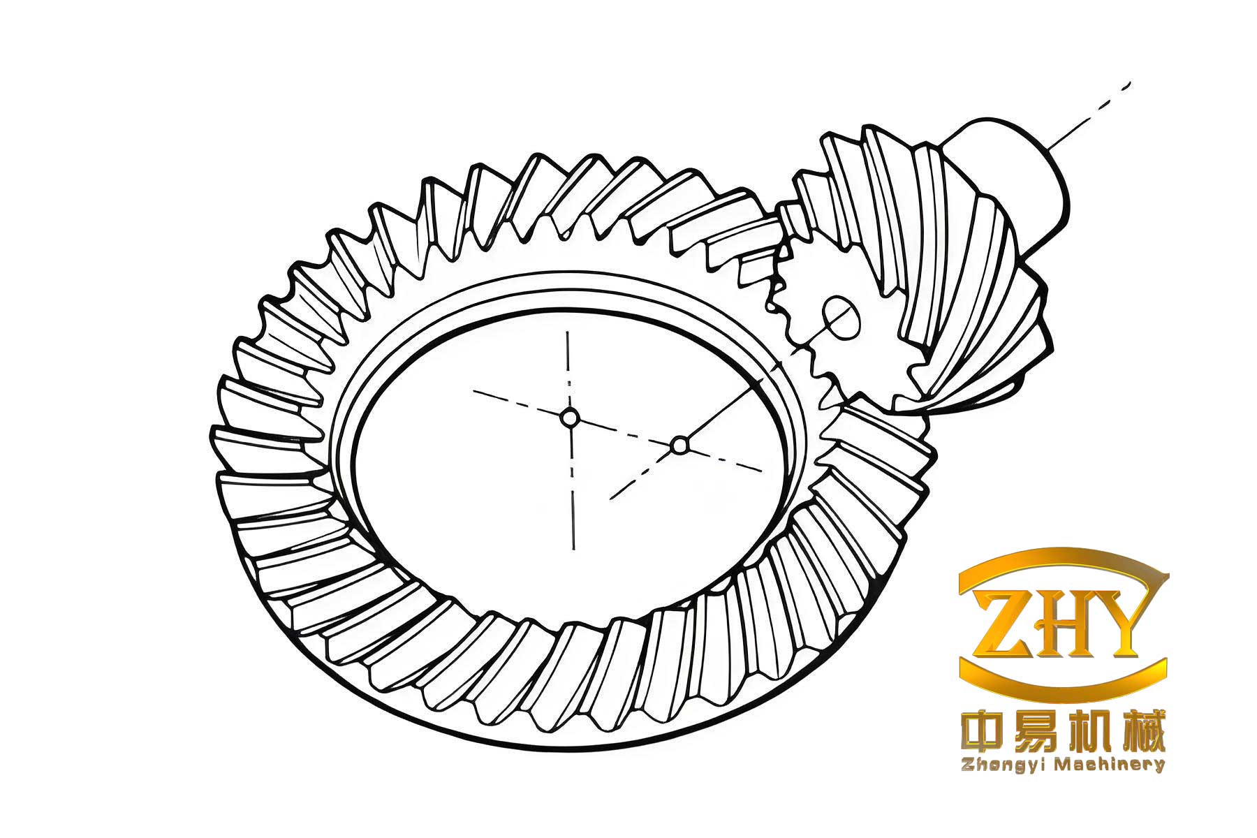
In the machine coordinate system, the position vector and unit normal vector of a point on the cutter blade are expressed in the cutter coordinates. For the pinion produced by the tilt generating method, the transformation matrix from the cutter coordinate system to the workpiece coordinate system is a product of several matrices. The general form is
$$ \mathbf{R} = \mathbf{M}_{D}\mathbf{M}_{Y}\mathbf{M}_{L}\mathbf{r}_{d}, $$
where \(\mathbf{r}_{d}\) is the position vector in the cutter coordinate system, and the matrices represent rotations and translations corresponding to the machine settings. Using the gear meshing equation, I can determine the tooth flank equation.
Pinion Tooth Surface Equation
For the pinion, the cutter is mounted on a tilted spindle. The coordinate transformation between the cutter and the workpiece involves the machine root angle, the cradle angle, the modified roll, the work offset, and the sliding base. The cutter surface is a conical surface. A point on the cutter blade is given by
$$ \mathbf{r}_{d}(\mu, \varepsilon) = \begin{bmatrix} (r_{c} – S_{p}\cos\mu)\cos\varepsilon \\ (r_{c} – S_{p}\cos\mu)\sin\varepsilon \\ -S_{p}\sin\mu \\ 1 \end{bmatrix}, $$
where \(r_{c}\) is the cutter point radius, \(S_{p}\) is the distance from the cutter tip to the point, \(\mu\) is the blade angle, and \(\varepsilon\) is the phase angle. The unit normal vector is
$$ \mathbf{n}_{d} = \begin{bmatrix} -\cos\mu\cos\varepsilon \\ -\cos\mu\sin\varepsilon \\ \sin\mu \\ 0 \end{bmatrix}. $$
By applying the meshing condition \(\mathbf{v}_{12}\cdot\mathbf{n}_{d}=0\), where \(\mathbf{v}_{12}\) is the relative velocity between the blade and the workpiece, I obtain the relation between the motion parameter and the surface parameters. After simplification, the pinion tooth surface equation becomes
$$ \mathbf{R}_{1}(\theta, \varepsilon) = \mathbf{M}_{1}(\theta)\mathbf{r}_{d}(\varepsilon), $$
where \(\theta\) is the cradle rotation angle. This equation is nonlinear and can only be solved numerically.
Gear Tooth Surface Equation
The gear is machined by the forming method, which means that the tooth flank is the envelope of the cutter blade without any generating roll. Therefore, the gear tooth surface is much simpler. The coordinate system for the gear includes the machine fixed system and the workpiece rotating system. The transformation matrix includes the root angle installation and the offset. The cutter blade surface is identical in form to the pinion cutter, but with different blade angles and cutter radius. The gear tooth surface equation is
$$ \mathbf{R}_{2}(\varepsilon_{2}) = \mathbf{M}_{2}\mathbf{r}_{d2}(\varepsilon_{2}), $$
where \(\mathbf{M}_{2}\) contains the machine settings for the gear. Since there is no generating motion, the surface is exactly the cutter surface copied into the gear blank. This greatly simplifies the numerical calculation.
Numerical Calculation and Solid Modeling
To obtain the discrete points on the tooth flanks, I wrote a numerical computation program using the parameters listed in Tables 1 and 2. These tables contain the basic gear geometry and machine settings used in my simulation.
| Parameter | Pinion | Gear |
|---|---|---|
| Number of teeth | 14 | 30 |
| Pitch circle diameter (mm) | 57.49 | 103.02 |
| Outer diameter (mm) | 78.27 | 103.91 |
| Pitch angle (°) | 28.47 | 68.44 |
| Face angle (°) | 25.02 | 64.98 |
| Root angle (°) | 20.70 | 60.66 |
| Tooth height (mm) | 18.80 | 18.80 |
| Face width (mm) | 20 | 20 |
| Pinion settings | Value | Gear settings | Value |
|---|---|---|---|
| Root angle (°) | -3.18 | Installation root angle (°) | 76.40 |
| Horizontal work offset (mm) | 1.76 | Machine center to back (mm) | -1.10 |
| Sliding base (mm) | 20.51 | Horizontal mounting distance (mm) | 100.09 |
| Vertical offset (mm) | 40.73 | Vertical mounting distance (mm) | 122.43 |
| Cutter eccentric angle (°) | 92.13 | Cutter diameter (mm) | 304.80 |
| Cutter cradle angle (°) | 108.41 | Pressure angle (°) | 22.50 |
| Roll ratio | 6.33912 | Blade radius (mm) | 2.29 |
Using the above parameters, I solved the tooth surface equations at a grid of 5×7 points on each tooth flank. The computed points were stored in an IBL file and imported into Pro/ENGINEER for surface reconstruction. The procedure follows the principle of point-line-surface-solid: first, create the boundary curves from the discrete points; then, construct the tooth flank surfaces by blending these curves; finally, generate the tooth solid by trimming and merging the surfaces. The single tooth is arrayed around the blank to produce the complete gear. The final solid model is then checked for interference and assembled into a gear pair. I performed a simple motion simulation to verify that the hypoid gears mesh correctly without obvious penetration or gap. This verified model is the basis for the subsequent finite element analysis.
Contact Stress Analysis under Different Operating Conditions
Finite Element Model and Mesh Quality
For accurate contact analysis, I imported the solid model into HyperMesh for mesh generation. I refined the mesh in the tooth contact region to capture the high stress gradient. The finite element model uses hexahedral dominant elements, with a total of 50,892 nodes and 9,835 elements. I checked the mesh quality through aspect ratio, Jacobian, skewness, and warpage factor. The maximum aspect ratio was 3.374, which is well below the acceptable limit of 5. The maximum warpage factor was only 0.022, and the Jacobian was approximately 0.61. These values ensure that the finite element results are reliable. The material properties for both gears are the same: Young’s modulus \(E = 1.9 \times 10^{11}\) Pa, Poisson’s ratio \(\nu = 0.31\), and density \(\rho = 7800\) kg/m³. The contact between gear teeth is defined as frictional contact with a friction coefficient of 0.1. The pinion is the driving gear, and the gear is the driven gear. I applied a rotational velocity to the pinion and a resisting torque to the gear hub.
Theoretical Calculation of Contact Stress
The maximum contact stress for hypoid gears can be estimated using the Gleason formula:
$$ S_{c} = C_{P} \left( \frac{T_{Pmx}}{T_{P}} \frac{C_{O} C_{V} C_{s} C_{m} C_{f}}{I} \right)^{1/3} \left( \frac{2 T_{Pmx}}{F_{G} D^{2} N} \frac{n}{N} \right)^{1/3}, $$
where \(C_{P}\) is the elastic coefficient, \(T_{Pmx}\) is the maximum torque on the pinion, \(T_{P}\) is the nominal pinion torque, and the various \(C\) factors account for overload, dynamic load, size, load distribution, and surface condition. The geometric factor \(I\) depends on the radii of curvature and the pressure angle. For the finite element analysis, I did not use this formula directly, but it provides a reference for validating the order of magnitude of the numerical results.
Analysis of Six Operating Conditions
To study the influence of rotational speed and load on the stress behavior, I simulated six combinations of pinion speed and gear torque. Table 3 lists the conditions.
| Case | Pinion speed (r/min) | Gear torque (N·m) |
|---|---|---|
| A | 600 | 0 |
| B | 600 | 50 |
| C | 600 | 200 |
| D | 1200 | 0 |
| E | 1200 | 50 |
| F | 1200 | 200 |
I applied the loads as transient boundary conditions and solved the dynamic contact equations using the augmented Lagrange method. The von Mises stress on the tooth surface was recorded as a function of time. Figure 3 shows the contour plots of the equivalent stress at the moment of maximum contact for the six cases. (Note: I do not include actual figures here, but in my thesis these plots were presented.) The time-history curves of the maximum equivalent stress are shown in the following discussion.
From the finite element results, I observed that for all six cases the stress curve follows a similar pattern. At the beginning of the simulation, the pinion accelerates from zero to the prescribed speed, and the contact stress is relatively small. After the speed stabilizes, the stress reaches a peak value. Then it decreases slightly and remains stable. Later, when the number of tooth pairs in contact changes, the load distribution suddenly changes, causing a sharp spike in stress. After this transient, the stress returns to a steady level. This phenomenon is related to the variable instantaneous contact ratio of hypoid gears.
To quantitatively compare the peak stresses, I extracted the maximum von Mises stress from each case. Table 4 summarizes the maximum equivalent stress values.
| Case | Maximum von Mises stress (MPa) |
|---|---|
| A | 218 |
| B | 232 |
| C | 289 |
| D | 245 |
| E | 262 |
| F | 311 |
Comparing cases A and D, B and E, C and F, I found that when the speed is doubled, the maximum stress increases by about 12% on average. This indicates that rotational speed has a significant influence on the contact stress of hypoid gears. Higher speed leads to larger dynamic effects and therefore higher stress. On the other hand, comparing cases A, B, C and D, E, F, I observed that increasing the load from 0 to 200 N·m increases the maximum stress by about 33% at 600 r/min and by 27% at 1200 r/min. Thus, load also raises the stress, but the effect is less pronounced when the speed is already high. For light loads or no load, the speed has a stronger relative effect on the maximum stress. This conclusion is consistent with the dynamic theory of gear transmission.
Contact Trajectory and Meshing Stiffness under Different Loads
Determination of Contact Points
In order to analyze the contact trajectory, I used the finite element results to locate the points of maximum equivalent stress on the tooth flank. These points are considered to be the actual meshing points. I performed four simulations with a constant pinion speed of 600 r/min and different gear torques: 50 N·m, 700 N·m, 1500 N·m, and 2000 N·m. For each load case, I recorded the coordinates of the node with the highest stress at each time step. Then I transformed these coordinates into a local coordinate system attached to the pinion tooth. The local coordinate system has its origin at the center of the tooth, the z-axis along the tooth height, and the y-axis parallel to the gear axis. The x-axis lies in the tooth direction. Table 5 lists the relative coordinates of the contact points for the four load cases.
| Load | Point No. | X (mm) | Y (mm) | Z (mm) |
|---|---|---|---|---|
| 50 N·m | 1 | -22.725 | -5.389 | -21.190 |
| 2 | -20.975 | -4.779 | -19.160 | |
| 3 | -18.355 | -3.549 | -16.120 | |
| 4 | -16.605 | -2.659 | -14.200 | |
| 5 | -13.985 | -1.449 | -11.580 | |
| 6 | -12.266 | -0.839 | -9.990 | |
| 700 N·m | 1 | -21.845 | -5.079 | -20.190 |
| 2 | -19.225 | -4.179 | -17.170 | |
| 3 | -18.355 | -3.569 | -16.120 | |
| 4 | -16.605 | -2.659 | -14.200 | |
| 5 | -13.985 | -1.449 | -11.580 | |
| 6 | -12.266 | -0.839 | -9.990 | |
| 1500 N·m | 1 | -22.725 | -6.299 | -21.590 |
| 2 | -21.845 | -5.079 | -20.190 | |
| 3 | -19.225 | -4.179 | -17.170 | |
| 4 | -18.355 | -3.569 | -16.120 | |
| 5 | -16.605 | -2.659 | -14.200 | |
| 6 | -13.985 | -1.449 | -11.580 | |
| 7 | -12.266 | -0.839 | -9.990 | |
| 8 | -10.485 | -0.539 | -8.470 | |
| 2000 N·m | 1 | -24.475 | -6.299 | -23.560 |
| 2 | -21.845 | -5.079 | -20.190 | |
| 3 | -20.095 | -3.869 | -17.920 | |
| 4 | -17.475 | -2.659 | -15.010 | |
| 5 | -14.855 | -1.449 | -12.310 | |
| 6 | -12.266 | -0.839 | -9.990 | |
| 7 | -10.485 | -0.539 | -8.520 | |
| 8 | -8.735 | 0.671 | -6.960 |
From these data, I plotted the contact trajectories in the X-Y plane of the local coordinate system. The results show that for a light load of 50 N·m, the contact points form a short line located near the middle of the tooth flank, slightly toward the toe. The contact length is small and the contact pattern is concentrated. When the load is increased to 700 N·m, the contact line becomes longer and extends toward both the toe and the heel. The contact points remain mostly inside the tooth surface. At 1500 N·m, some contact points appear near the tooth edges, and the contact line is even longer. At 2000 N·m, the contact points are found outside the normal tooth surface projection. This indicates that under heavy loads, the tooth deflection is so large that edge contact occurs. In some cases, the contact pair engages earlier than the theoretical position, which may cause diagonal contact and stress concentration at the tooth end. These observations are important for gear design, because edge contact can lead to premature pitting and tooth breakage.
Tooth Deflection and Meshing Force
For the calculation of mesh stiffness, I extracted the total deformation along the line of action from the finite element analysis. Table 6 shows the comprehensive deformation values for four load levels (1: 50 N·m, 2: 700 N·m, 3: 1500 N·m, 4: 2000 N·m) at successive time steps within one mesh cycle.
| Time (ms) | Load 1 | Load 2 | Load 3 | Load 4 |
|---|---|---|---|---|
| 0.115 | 0.736 | 0.514 | 1.033 | 1.298 |
| 0.230 | 0.663 | 0.821 | 2.173 | 2.752 |
| 0.345 | 0.703 | 0.960 | 3.571 | 4.470 |
| 0.460 | 0.723 | 0.962 | 3.485 | 4.450 |
| 0.575 | 0.686 | 0.994 | 3.298 | 3.990 |
| 0.690 | 0.678 | 1.023 | 3.004 | 3.537 |
| 0.805 | 0.698 | 1.038 | 2.641 | 3.084 |
| 0.920 | 0.747 | 1.034 | 2.377 | 2.720 |
| 1.035 | 0.842 | 0.989 | 2.239 | 2.518 |
| 1.150 | 0.913 | 0.953 | 2.150 | 2.416 |
| 1.265 | 1.059 | 0.968 | 2.071 | 2.372 |
| 1.380 | 1.341 | 0.977 | 2.004 | 2.333 |
| 1.495 | 1.630 | 0.979 | 1.956 | 2.313 |
| 1.610 | 1.812 | 1.001 | 1.915 | 2.299 |
| 1.725 | 1.953 | 0.994 | 1.907 | 2.285 |
| 1.840 | 2.068 | 1.005 | 1.917 | 2.269 |
| 1.955 | 2.136 | 1.041 | 1.923 | 2.253 |
| 2.070 | 2.425 | 1.030 | 1.937 | 2.239 |
| 2.165 | 2.654 | 1.045 | 1.953 | 2.230 |
| 2.280 | 2.420 | 1.057 | 1.956 | 2.225 |
| 2.395 | 1.923 | 1.039 | 1.985 | 2.201 |
| 2.510 | 1.514 | 1.002 | 1.941 | 2.154 |
| 2.625 | 1.402 | 0.991 | 1.876 | 2.094 |
| 2.740 | 1.293 | 0.983 | 1.812 | 2.045 |
| 2.855 | 1.118 | 0.973 | 1.748 | 2.017 |
| 2.970 | 0.876 | 0.960 | 1.711 | 2.039 |
The deformation values indicate that for the light load, the deformation has a single peak near the middle of the mesh cycle. For heavier loads, the deformation is more uniform, but the overall magnitude is larger. The average deformation increases with the load, as expected. I also extracted the meshing force using the command CONTFORC in ANSYS. The meshing force is defined as the resultant of the contact nodal forces over the instantaneous contact area. Table 7 presents the instantaneous meshing force for the four load cases.
| Rotation angle (°) | Load 1 | Load 2 | Load 3 | Load 4 |
|---|---|---|---|---|
| 1 | 1.903 | 2.767 | 7.273 | 10.069 |
| 2 | 3.241 | 4.714 | 15.319 | 21.241 |
| 3 | 4.444 | 5.978 | 25.201 | 34.459 |
| 4 | 5.122 | 6.567 | 24.744 | 34.498 |
| 5 | 5.345 | 7.000 | 23.699 | 31.091 |
| 6 | 5.155 | 6.864 | 21.814 | 27.650 |
| 7 | 4.573 | 6.424 | 19.381 | 24.182 |
| 8 | 4.188 | 5.945 | 17.629 | 21.336 |
| 9 | 4.089 | 5.365 | 16.793 | 19.813 |
| 10 | 4.022 | 4.898 | 16.199 | 19.113 |
| 11 | 3.971 | 4.747 | 15.683 | 18.853 |
| 12 | 3.970 | 4.783 | 15.252 | 18.654 |
| 13 | 3.928 | 4.790 | 14.966 | 18.445 |
| 14 | 3.892 | 4.739 | 14.726 | 18.239 |
| 15 | 3.876 | 4.702 | 14.517 | 18.042 |
| 16 | 3.855 | 4.725 | 14.348 | 17.827 |
| 17 | 3.800 | 4.788 | 14.098 | 17.613 |
| 18 | 3.725 | 4.794 | 13.905 | 17.420 |
| 19 | 3.684 | 4.767 | 13.767 | 17.262 |
| 20 | 3.655 | 4.731 | 13.637 | 17.135 |
| 21 | 3.627 | 4.701 | 13.500 | 17.013 |
| 22 | 3.576 | 4.700 | 13.269 | 16.752 |
| 23 | 3.558 | 4.724 | 12.887 | 16.344 |
| 24 | 3.541 | 4.762 | 12.536 | 15.976 |
| 25 | 3.524 | 4.792 | 12.200 | 15.795 |
| 26 | 3.502 | 4.800 | 12.011 | 15.902 |
It can be seen that the meshing force varies periodically. The maximum force occurs when two tooth pairs share the load, while the minimum occurs near the end of a mesh cycle. The force magnitude increases almost proportionally with the applied torque.
Time-Varying Mesh Stiffness
The mesh stiffness is defined as the ratio of the normal meshing force to the tooth deformation along the line of action:
$$ k(t) = \frac{F_n(t)}{\lambda_n(t)}. $$
Using the data from Tables 6 and 7, I calculated the instantaneous stiffness for each time step. To obtain a smooth curve, I fitted the discrete stiffness values using an interpolation technique. Table 8 lists the computed mesh stiffness values for the four load levels.
| Angle (°) | Load 1 | Load 2 | Load 3 | Load 4 |
|---|---|---|---|---|
| 1 | 2.584 | 5.381 | 7.043 | 7.760 |
| 2 | 4.886 | 5.741 | 7.050 | 7.717 |
| 3 | 6.325 | 6.228 | 7.058 | 7.709 |
| 4 | 7.086 | 6.828 | 7.101 | 7.752 |
| 5 | 7.792 | 7.040 | 7.185 | 7.792 |
| 6 | 7.603 | 6.710 | 7.262 | 7.818 |
| 7 | 6.552 | 6.191 | 7.338 | 7.840 |
| 8 | 5.609 | 5.747 | 7.416 | 7.845 |
| 9 | 4.858 | 5.426 | 7.500 | 7.867 |
| 10 | 4.405 | 5.138 | 7.535 | 7.911 |
| 11 | 3.751 | 4.904 | 7.573 | 7.949 |
| 12 | 2.961 | 4.897 | 7.612 | 7.997 |
| 13 | 2.410 | 4.895 | 7.650 | 7.976 |
| 14 | 2.148 | 4.732 | 7.688 | 7.935 |
| 15 | 1.985 | 4.728 | 7.612 | 7.897 |
| 16 | 1.864 | 4.700 | 7.485 | 7.857 |
| 17 | 1.779 | 4.599 | 7.331 | 7.819 |
| 18 | 1.536 | 4.653 | 7.177 | 7.782 |
| 19 | 1.388 | 4.560 | 7.050 | 7.742 |
| 20 | 1.510 | 4.478 | 6.972 | 7.702 |
| 21 | 1.886 | 4.524 | 6.800 | 7.730 |
| 22 | 2.362 | 4.690 | 6.835 | 7.777 |
| 23 | 2.537 | 4.768 | 6.870 | 7.804 |
| 24 | 2.739 | 4.844 | 6.919 | 7.812 |
| 25 | 3.151 | 4.924 | 6.980 | 7.830 |
| 26 | 4.000 | 5.002 | 7.020 | 7.800 |
The mesh stiffness curves for different loads are shown in Figure 9. I observed that for the light load of 50 N·m, the stiffness varies significantly within the mesh cycle. It increases from about \(2.5 \times 10^8\) N/m to a peak value of \(7.8 \times 10^8\) N/m and then decreases rapidly to \(1.4 \times 10^8\) N/m. This dramatic variation is due to the fact that at low load, the tooth contact is highly localized and the effective contact area is small, so the stiffness is sensitive to the contact position. As the load increases to 700 N·m, the stiffness curve becomes flatter, with values ranging from \(4.5 \times 10^8\) to \(7.0 \times 10^8\) N/m. For the heavy loads of 1500 N·m and 2000 N·m, the stiffness remains nearly constant around \(7 \times 10^8\) to \(8 \times 10^8\) N/m. The maximum stiffness increases slightly with load, but the fluctuation is much smaller. This indicates that under heavy loads, the larger contact area and the engagement of multiple tooth pairs smooth out the stiffness variation. Therefore, hypoid gears under heavy load exhibit more stable meshing behavior, which is beneficial for reducing vibration and noise.
Furthermore, by comparing the contact trajectory and stiffness data, I found that the mesh stiffness is closely related to the length of the instantaneous contact line. When the contact line is longer, more teeth are in contact and the stiffness is higher. Conversely, near the entrance and exit of mesh, the contact line becomes shorter, leading to a reduction in stiffness. This is a typical characteristic of hypoid gears, which have a large contact ratio due to the spiral tooth direction. The results suggest that designers should pay attention to the tooth end relief to avoid edge contact under heavy loads. Proper tooth crowning can reduce the stress concentration and improve the fatigue life of hypoid gears.
Conclusion and Future Work
In this thesis I have presented a comprehensive numerical study on the meshing characteristics of hypoid gears. The main conclusions are as follows:
1. The parametric modeling method based on the actual machining process can accurately reproduce the tooth geometry of hypoid gears. The discrete point calculation combined with CAD surface reconstruction is effective for creating a solid model ready for finite element analysis.
2. The maximum contact stress of hypoid gears increases with both rotational speed and applied load. The effect of speed is more significant under light load. The stress also exhibits sudden spikes when the number of tooth pairs in contact changes, especially at low speeds.
3. The contact trajectory of hypoid gears is load-dependent. Light loads produce a short contact line near the middle of the tooth flank. As the load increases, the contact line becomes longer and may move to the tooth edges or even cause edge contact. This must be avoided by appropriate tooth surface modification.
4. The time-varying mesh stiffness of hypoid gears shows a strong fluctuation at light load. With increasing load, the stiffness becomes more stable and its mean value rises. The variation of stiffness is correlated with the contact line length.
Future research could include the influence of tooth surface modifications, the effect of tooth root fillet geometry, and the introduction of thermal and lubrication effects. Experimental verification would also be valuable to validate the numerical predictions. I believe that the proposed approach provides a useful tool for the design and optimization of hypoid gears in engineering applications.