
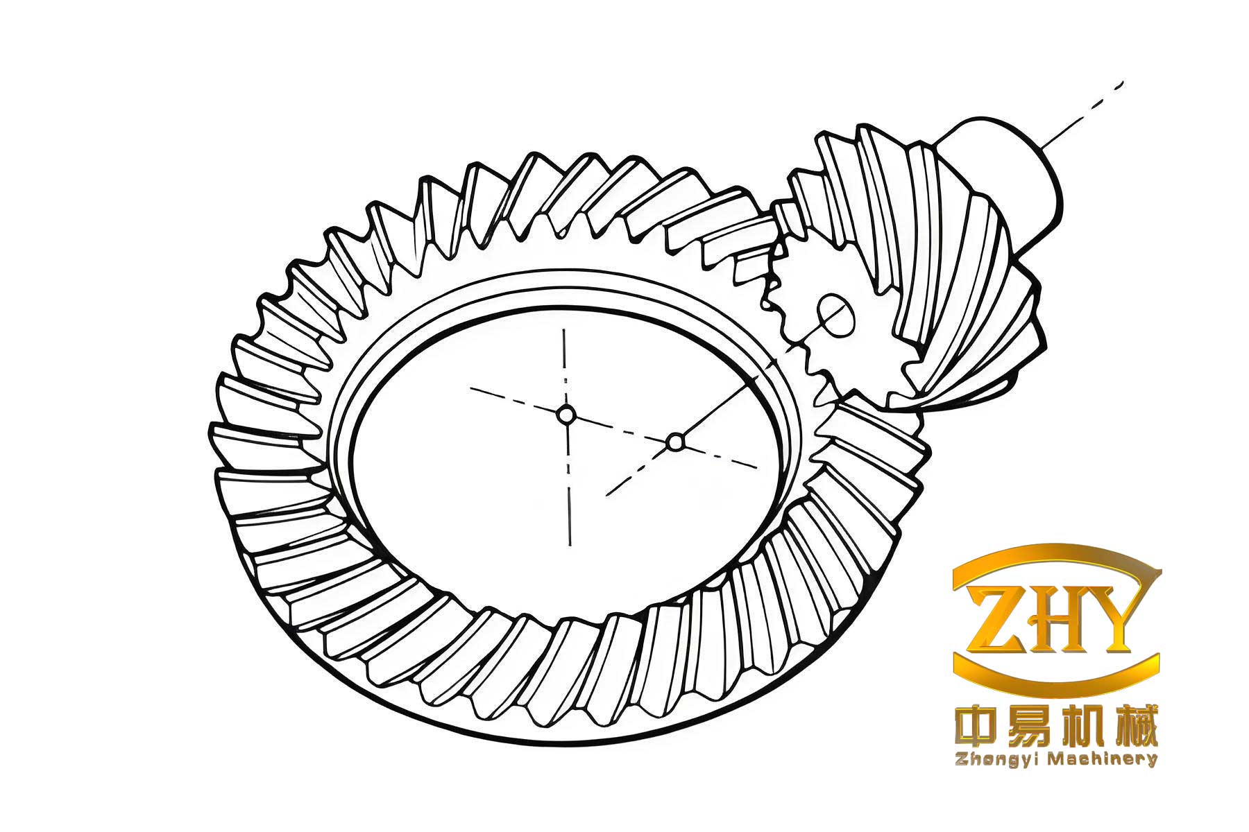
Hypoid gear transmission possesses a series of advantages such as large contact ratio, strong load-carrying capacity, high transmission efficiency, smooth transmission, low noise, and large reduction ratio. It can be used to transmit motion and power between two crossed-axis shafts. Due to the existence of the pinion offset, it is widely applied in mechanical transmission devices that have special space requirements, such as automotive drive axles. The time-varying nature of the gear pair mesh stiffness induces periodic vibrations in the transmission system. Therefore, developing an efficient and accurate calculation method for the time-varying mesh stiffness of hypoid gear pairs and analyzing its influencing factors constitute an important research direction, which holds significant theoretical significance and engineering practical value for improving the dynamic performance of hypoid gear transmission.
In this research, the Gleason modified roll method (HGM) hypoid gear is investigated comprehensively. The main research contents include gear pair solid modeling, tooth contact analysis (TCA), loaded tooth contact analysis (LTCA), time-varying mesh stiffness calculation, and the influence analysis of pinion machine tool settings on the time-varying mesh stiffness and dynamic performance. The research work presented in this thesis is structured as follows.
1. Introduction and Research Background
Hypoid gears are among the most complex gear types in terms of contact mechanism and machining principles. Compared with ordinary cylindrical gear transmissions, hypoid gear drives offer superior characteristics including large contact ratio, high load capacity, high transmission efficiency, stable operation, low noise, and large speed reduction ratios. Since the invention of the first spiral bevel gear cutting machine by Gleason in 1913, hypoid gear transmission technology has matured considerably. However, the engineering demands on transmission performance continue to increase, making the improvement of hypoid gear dynamic performance an important research topic.
The two tooth flanks of hypoid gears are asymmetric spatially complex curved surfaces. The paired tooth surfaces exhibit localized point-contact conjugation. The tooth contact pattern varies with machine tool settings, and the position and size of the contact pattern not only affect the load-carrying capacity and service life of the gear pair but also influence transmission vibration and noise. During gear transmission, the variation of meshing position causes the mesh stiffness to change with time. The time-varying mesh stiffness is a primary component of the internal excitation of the system and is one of the sources of vibration and noise. Therefore, for hypoid gear transmission, it is essential not only to study the tooth contact characteristics but also to conduct research on the calculation methods and influencing factors of time-varying mesh stiffness, as well as the influence of machine tool settings on the system dynamic performance.
This research focuses on the HGM hypoid gear pair manufactured by the Gleason method. The tooth surface equations of the gear and pinion are derived from the generating tool surfaces. Based on the tooth surface equations, a solid model of the gear pair is established. Combined with the point-contact conjugate contact theory, a tooth contact analysis (TCA) mathematical model is developed to investigate the contact pattern under ideal unloaded conditions. On the basis of TCA, considering the deformation of gear teeth under load, a loaded tooth contact analysis (LTCA) model is established. Combined with the classical Hertzian point contact theory, the time-varying mesh stiffness of the gear pair is derived and compared with finite element calculation results. The influence laws of pinion machine tool settings, such as tooth height curvature correction coefficient, generating gear cone pitch, vertical offset, and radial tool position, on the time-varying mesh stiffness are analyzed. Based on the lumped parameter method, a dynamic model of hypoid gear transmission considering comprehensive time-varying mesh stiffness, transmission error, and backlash is established to study the influence of pinion machine tool settings on the dynamic performance of the hypoid gear transmission system.
2. Literature Review
Extensive research has been conducted by scholars worldwide on hypoid gear contact analysis. As early as 1961, Baxter and colleagues first proposed the basic theoretical method of tooth contact analysis, combined with computer technology to solve complex contact problems, and predicted the contact path of hypoid gear pairs. In 1978, Gleason Works published a relatively complete principle and method of tooth contact analysis, providing calculation methods for the orientation and size of the tooth contact ellipse under light loads. Subsequently, edge tooth contact analysis was developed. In 2007, Fan improved the original TCA theory by adopting a two-layer iterative algorithm that enhanced the accuracy of contact pattern simulation. In 2008, Tang Jinyuan incorporated various machine tool errors and gear pair installation errors into the contact mathematical model, proposing error tooth contact analysis.
In 1981, Krenzer considered the elastic deformation of gear teeth under load and first proposed the theoretical method of loaded tooth contact analysis, which can calculate the contact pattern, geometric transmission error curve, contact ratio, and load distribution among teeth of spiral bevel gears under load. In 1993, Zheng Changqi developed an LTCA model for spiral bevel gears by treating the deformation of the gear pair support system caused by load as installation adjustments. In 1996, Litvin performed LTCA for spiral bevel gears using finite element methods. In 1998, Fang Zongde proposed an LTCA method based on the tooth surface compliance matrix and applied it to spiral bevel gears and modified helical gears. In 2001, Simon studied the influence of machine tool setting changes on the dynamic performance during loaded transmission, obtaining machine tool settings that yield ideal dynamic performance.
Regarding time-varying mesh stiffness calculation, Cornell simplified gears as cantilever beam models in 1981. In 1994, Liu Geng used finite element methods to calculate the mesh stiffness of internal and external gear pairs. In 2000, Lin Tengjiao established precise finite element contact analysis models for helical gear pairs at arbitrary meshing positions. In 2008, Bu Zhonghong extracted the tooth surface compliance matrix of helical gears using finite element methods and solved for gear mesh stiffness and tooth surface load distribution using linear programming methods. In 2010, Li Yapeng improved the Ishikawa time-varying mesh stiffness calculation formula by considering the influence of the gear body. In 2011, Chen and Shao comprehensively considered contact, bending, shear, compression deformation, and base deformation of gear teeth to calculate spur gear mesh stiffness. In 2014, Ma and colleagues proposed an improved time-varying mesh stiffness calculation method for cracked spur gears. In 2017, Liu Cheng performed loaded contact finite element analysis on hypoid gears, considering the influence of the gear meshing force direction changing with meshing position, thereby improving the calculation accuracy of hypoid gear mesh stiffness.
For gear transmission system dynamic response research, Kahraman and Singh established a three-degree-of-freedom gear-rotor-bearing dynamic model in 1991. In 1999, Cheng and Lim predicted the natural frequencies and mode shapes of hypoid gear systems. In 2003, Li and Hu studied the coupled vibration mechanism of spiral bevel gears. In 2007, Wang established a time-varying mesh stiffness model for hypoid gears and performed dynamic analysis. In 2011, Lin Tengjiao considered gear tooth contact deformation, shaft bending deformation, and bearing deformation to predict the dynamic response of hypoid gearboxes using finite element methods. In 2012, Yang improved the multi-term harmonic balance method to predict harmonic and subharmonic responses of hypoid gear systems.
3. Hypoid Gear Modeling and Tooth Contact Analysis
3.1 Cutting Principles and Methods of Hypoid Gears
Gleason hypoid gears are machined on gear cutting machines. The rotating cutter head on the machine oscillates with the cradle mechanism to form an imaginary gear. The relative motion between the workpiece and the imaginary gear can be regarded as a pair of hypoid gears meshing. The cutting surface of the imaginary gear and the machined tooth surface satisfy the conjugate condition. This machining method is called the generating method, and the imaginary gear formed by the combined motion of the cradle and cutter head is called the generating gear.
There are generally two forms of generating gears: the plane generating gear and the conical generating gear. The plane generating gear has a face cone angle of 90 degrees, which is mainly used for machining large gears and pinions by the modified roll method. Hypoid gear large gears are typically machined by the generating method or the forming method. The generating method is based on the plane generating gear principle with a constant ratio between the generating gear and workpiece, suitable for large gears with root angles less than 70 degrees. The forming method cuts the tooth directly without relative motion between the cutter and workpiece, suitable for large gears with root angles greater than 70 degrees.
Hypoid gear pinions are typically machined by the modified roll method or the tilt method. The modified roll method is based on the plane generating gear principle with a varying ratio between the generating gear and workpiece. The tilt method is based on the conical generating gear principle with a constant transmission ratio but an inclined cutter spindle.
3.2 Tooth Surface Equations
Based on the gear meshing principle and spatial transformation matrices, the tooth surface equations of the gear and pinion are derived from the generating tool surface equations. According to the Gleason hypoid gear cutting machine layout, coordinate systems representing each machine mechanism are established. Meanwhile, the coordinate transformation matrices from the tool coordinate system to the workpiece coordinate system are derived.
The tool coordinate system to cradle coordinate system transformation matrix is expressed as:
$$ \mathbf{M}_{gt} = \begin{bmatrix} 1 & 0 & 0 & \mp S\cos q \\ 0 & 1 & 0 & \pm S\sin q \\ 0 & 0 & 1 & 0 \\ 0 & 0 & 0 & 1 \end{bmatrix} $$
where \(S\) is the radial tool position and \(q\) is the angular tool position. The “±” sign is taken as “-” when machining left-hand gears and “+” when machining right-hand gears.
The cradle coordinate system to machine coordinate system transformation matrix is:
$$ \mathbf{M}_{og} = \begin{bmatrix} \cos\phi_g & -\sin\phi_g & 0 & 0 \\ \sin\phi_g & \cos\phi_g & 0 & 0 \\ 0 & 0 & 1 & 0 \\ 0 & 0 & 0 & 1 \end{bmatrix} $$
The machine coordinate system to auxiliary coordinate system transformation matrix is:
$$ \mathbf{M}_{fo} = \begin{bmatrix} 1 & 0 & 0 & X\sin\gamma \\ 0 & 1 & 0 & -E_o \\ 0 & 0 & 1 & -(X\cos\gamma + X_B) \\ 0 & 0 & 0 & 1 \end{bmatrix} $$
where \(X\) is the axial wheel position, \(X_B\) is the bed position, \(E_o\) is the vertical offset, and \(\gamma\) is the workpiece installation angle.
The auxiliary coordinate system to workpiece coordinate system transformation matrix is:
$$ \mathbf{M}_{pa} = \begin{bmatrix} 1 & 0 & 0 & 0 \\ 0 & \cos\phi_p & \sin\phi_p & 0 \\ 0 & -\sin\phi_p & \cos\phi_p & 0 \\ 0 & 0 & 0 & 1 \end{bmatrix} $$
For the inner cutting edge of the pinion cutter, the generating cone surface equation in the tool coordinate system is:
$$ \mathbf{r}_t^{11}(u_{11}, \theta_{1i}) = \begin{bmatrix} (r_{1i} – u_{11}(1-\sin\alpha_{1i})\tan\alpha_{1i}\sin\alpha_{1i})\cos\theta_{1i} \\ (r_{1i} – u_{11}(1-\sin\alpha_{1i})\tan\alpha_{1i}\sin\alpha_{1i})\sin\theta_{1i} \\ u_{11}(1-\sin\alpha_{1i})\cos\alpha_{1i} \\ 1 \end{bmatrix} $$
By applying the coordinate transformations and the meshing equation \(\mathbf{n} \cdot \mathbf{v} = 0\), the tooth surface equations of the pinion and gear can be derived.
3.3 Tooth Contact Analysis Mathematical Model
According to the gear meshing principle, the two tooth surfaces satisfy the conjugate contact condition when their position vectors and normal vectors are equal. The tooth contact analysis mathematical model is established as:
$$ \begin{cases} \mathbf{R}_1^m(u_1, \theta_1, \phi_1) = \mathbf{R}_2^m(u_2, \theta_2, \phi_2) \\ \mathbf{N}_1^m(u_1, \theta_1, \phi_1) = \mathbf{N}_2^m(u_2, \theta_2, \phi_2) \end{cases} $$
The TCA nonlinear equations contain six unknowns: \(u_1\), \(\theta_1\), \(\phi_1\), \(u_2\), \(\theta_2\), \(\phi_2\). To make the contact equations solvable, the pinion rotation angle \(\phi_1\) is selected as a known parameter, with different \(\phi_1\) values corresponding to different meshing positions of the gear pair. An initial meshing position needs to be determined first, and then other meshing positions can be solved by incrementing or decrementing \(\phi_1\).
For the initial value determination of TCA nonlinear equations, a method based on discrete tooth surface points is adopted. The pair of points with minimum spatial distance among all tooth surface point combinations after rotating around their respective axes is used as the initial value for solving the TCA equations.
The contact ellipse parameters are determined based on the limit normal curvature and its corresponding direction. The major semi-axis length \(l_1’\) and minor semi-axis length \(l_2’\) of the contact ellipse can be expressed as:
$$ l_1′ = \sqrt{\frac{2\delta}{\Delta K_{min}}} $$
$$ l_2′ = \sqrt{\frac{2\delta}{\Delta K_{max}}} $$
A numerical example of the TCA result is shown in Figure 2.20 of the original thesis, which demonstrates the contact path on the tooth surface.
3.4 Solid Model Construction
Based on the tooth surface equations, discrete point coordinates on the tooth surfaces are obtained by solving the equations in Matlab. The point clouds are imported into Imageware software for tooth surface fitting. Then, tooth surface patches are used in UG software to create the complete hypoid gear solid model. The gear pair is assembled according to the TCA analysis results. Figure 2.23 shows the solid models of the pinion and gear, and Figure 2.24 shows the assembled hypoid gear pair.
4. Time-varying Mesh Stiffness Calculation of Hypoid Gear Pair
4.1 Loaded Tooth Contact Analysis
For the LTCA of hypoid gears, the contact ellipse under load is simplified as a line coinciding with the major axis of the ellipse. Each continuous contact line is discretized into several contact points for subsequent analysis.
The deformation compatibility condition at any contact point \(i\) can be expressed as:
$$ u_i^{(1)} + u_i^{(2)} + \varepsilon_i = x_s + d_i $$
where \(\varepsilon_i\) is the initial clearance at contact point \(i\), \(d_i\) is the remaining clearance at contact point \(i\), \(x_s\) is the approach of the two elastic bodies, and \(u_i^{(1)}\), \(u_i^{(2)}\) are the bending-shear deformations of the pinion and gear at contact point \(i\), respectively.
The bending-shear deformations are linearly related to the loads:
$$ u_i^{(1)} = \sum_{j=1}^{n} \eta_{ij}^{(1)} F_j $$
$$ u_i^{(2)} = \sum_{j=1}^{n} \eta_{ij}^{(2)} F_j $$
where \(\eta_{ij}^{(1)}\) and \(\eta_{ij}^{(2)}\) are the bending-shear compliance coefficients, and \(F_j\) is the normal load at contact point \(j\).
The single-tooth pair loaded contact equation system at any meshing position can be written as:
$$ \begin{cases} [\lambda]_{\phi_1} \{F\}_{\phi_1} + \{\varepsilon\}_{\phi_1} = \{x_s\}_{\phi_1} + \{d\}_{\phi_1} \\ [1 \; 1 \; \cdots \; 1]\{F\}_{\phi_1} = P \end{cases} $$
For multiple tooth pairs in simultaneous contact, the loaded contact equations are extended accordingly. The iterative algorithm for solving the contact equations is shown in Figure 3.6 of the original thesis. In the first iteration, all contact points are assumed to be in contact. Then, the rows and columns with negative loads are eliminated, and the reduced equations are solved again until all remaining contact points satisfy the contact conditions.
4.2 Contact Point Bending-Shear Compliance Matrix
The normal bending-shear compliance matrix of the contact points is obtained using the finite element method. In this research, the substructure method in ANSYS is employed to extract the normal stiffness matrix of the tooth surface mesh nodes, which is then inverted to obtain the compliance matrix. The finite element model is shown in Figure 3.4, where both the gear and pinion contain only five teeth to reduce computational effort.
The compliance matrix of the contact points is obtained by interpolating the compliance matrix of the tooth surface mesh nodes. The griddata function in Matlab is used for interpolation. The interpolation is performed in two steps: first, interpolate the compliance coefficients of the mesh nodes with respect to the contact points; then, interpolate the compliance coefficients of the contact points with respect to each other.
4.3 Mesh Stiffness Calculation Based on LTCA
After solving the loaded contact equations, the normal load vector \(\{F\}\) and the corresponding bending-shear compliance matrix \([\lambda]\) of the actual contact points are obtained. The bending-shear deformation vector at any meshing position is:
$$ \{u_b\} = [\lambda]\{F\} $$
The bending-shear stiffness of the gear teeth at any meshing position is:
$$ k_b = \frac{\sum_{i=1}^{n} F_i}{\sum_{i=1}^{n} u_{bi}} $$
According to Hertzian contact theory, the Hertzian contact deformation can be expressed as:
$$ \delta_h = \frac{\pi c_\delta (A+B)P}{b} $$
The equivalent stiffness due to Hertzian contact deformation is:
$$ k_h = \frac{P}{\delta_h} = \frac{b}{\pi c_\delta (A+B)} $$
where \(A\) and \(B\) are parameters determined by the principal curvatures and principal directions of the contacting tooth surfaces, \(b\) is the minor semi-axis length of the contact ellipse, and \(c_\delta\) is the deformation coefficient.
The single-tooth mesh stiffness can be regarded as a series connection of the bending-shear stiffness spring and the Hertzian contact stiffness spring:
$$ k_m = \frac{k_h k_b}{k_h + k_b} $$
Figure 3.10 shows the single-tooth mesh stiffness and comprehensive mesh stiffness of the example hypoid gear pair based on LTCA.
4.4 Verification with Finite Element Method
To verify the accuracy of the LTCA-based method, the finite element method is also used to calculate the mesh stiffness. A finite element model of the hypoid gear pair with five teeth on each gear is established. The full displacement constraint is applied on the inner ring surface of the driven gear, and the radial and axial displacement constraints are applied on the inner ring surface of the driving gear while releasing the tangential degree of freedom. The tooth contact is simulated by adding contact pair elements on the tooth surfaces, and the transmitted torque is converted into tangential forces applied to the nodes on the inner ring surface of the pinion.
The comparison between the finite element method and the LTCA-based method results is shown in Figure 3.13. The figures indicate that although there are slight numerical differences between the two methods, the stiffness curve patterns are consistent, thus verifying the correctness of the LTCA-based method.
5. Influence of Machine Tool Settings on Time-varying Mesh Stiffness
In hypoid gear transmission, many factors influence the time-varying mesh stiffness, including gear design parameters, such as tooth number, module, pressure angle, and spiral angle, as well as machine tool settings, such as tooth height curvature correction coefficient, generating gear cone pitch, vertical offset, and radial tool position. Unlike involute cylindrical gears whose tooth geometry is fully determined once design parameters are fixed, hypoid gears have many combinations of machine tool settings that satisfy the same design parameters, each producing slightly different tooth geometry. Consequently, studying the influence of machine tool settings on time-varying mesh stiffness has more practical significance.
Generally, the pinion has more machine tool settings than the gear and exerts more effective control over the contact pattern. Moreover, since the pinion has fewer teeth, machine tool settings are typically selected for adjustment on the pinion. When a certain machine tool setting of the pinion is adjusted, the pinion tooth geometry changes, and the time-varying mesh stiffness changes accordingly. This chapter investigates the influence of HGM pinion machine tool settings—specifically the tooth height curvature correction coefficient, generating gear cone pitch, vertical offset, and radial tool position—on the time-varying mesh stiffness of hypoid gears.
5.1 Influence of Tooth Height Curvature Correction Coefficient
The adjustment value sequence of the tooth height curvature correction coefficient is shown in Table 5.1.
| No. | 1 | 2 | 3 | 4 | 5 |
|---|---|---|---|---|---|
| ΔKp | -0.15 | 0 | 0.15 | 0.3 | 0.45 |
For each adjustment value, the time-varying mesh stiffness and loaded contact pattern are calculated using the LTCA method. The comparison of the time-varying mesh stiffness for different \(\Delta K_p\) values is shown in Figure 4.6. As the tooth height curvature correction coefficient of the pinion increases, both the single-tooth mesh stiffness and the comprehensive mesh stiffness increase, and the meshing interval of the gear teeth increases. At the same time, both the pinion contact pattern and the gear contact pattern move toward the heel end of the tooth. The gear tooth at the heel end is thicker and has stronger resistance to deformation, resulting in the increasing trend of mesh stiffness.
5.2 Influence of Generating Gear Cone Pitch
The adjustment value sequence of the generating gear cone pitch is shown in Table 5.2.
| No. | 1 | 2 | 3 | 4 | 5 |
|---|---|---|---|---|---|
| ΔR01/mm | -0.2 | 0 | 0.2 | 0.4 | 0.6 |
Figure 4.12 presents the comparison of time-varying mesh stiffness for different \(\Delta R_{01}\) values. The results show that as the generating gear cone pitch increases, both the single-tooth mesh stiffness and the comprehensive mesh stiffness increase, and the meshing interval of the gear teeth increases. Meanwhile, both the pinion and gear contact patterns shift toward the heel end of the tooth. Since the tooth at the heel end is thicker, the load resistance capability is enhanced, and the mesh stiffness exhibits a growing trend.
5.3 Influence of Vertical Offset
The adjustment value sequence of the vertical offset is shown in Table 5.3.
| No. | 1 | 2 | 3 | 4 | 5 |
|---|---|---|---|---|---|
| ΔE01/mm | -0.5 | 0 | 0.5 | 1 | 1.5 |
Figure 4.18 displays the comparison of time-varying mesh stiffness for different \(\Delta E_{01}\) values. As the vertical offset of the pinion increases, both the single-tooth mesh stiffness and the comprehensive mesh stiffness decrease, while the meshing interval of the gear teeth increases. Simultaneously, the contact patterns of both the pinion and gear shift toward the toe end of the tooth. The gear tooth at the toe end is thinner with weaker deformation resistance, leading to the decreasing trend of mesh stiffness.
5.4 Influence of Radial Tool Position
The adjustment value sequence of the radial tool position is shown in Table 5.4.
| No. | 1 | 2 | 3 | 4 | 5 |
|---|---|---|---|---|---|
| ΔS1/mm | -0.15 | -0.1 | 0 | 0.1 | 0.2 |
Figure 4.24 shows the comparison of time-varying mesh stiffness for different \(\Delta S_1\) values. As the radial tool position of the pinion increases, both the single-tooth mesh stiffness and the comprehensive mesh stiffness decrease, and the meshing interval of the gear teeth increases. The contact patterns of both the pinion and gear shift toward the toe end of the tooth. With thinner tooth sections toward the toe end, the deformation resistance is weakened, and the mesh stiffness shows a decreasing trend.
6. Influence of Machine Tool Settings on Dynamic Performance
6.1 Dynamic Model of Hypoid Gear Transmission System
Based on the lumped parameter method, a bending-torsional-axial coupled vibration analysis model of the hypoid gear transmission is established. The gear pair is treated as mass points, with springs and dampers simulating the meshing of gears, and bearings simplified as springs and dampers supporting the gears.
In the dynamic model, ignoring friction between tooth surfaces, each gear has four degrees of freedom in space, and the entire transmission system has a total of 8 degrees of freedom. These include the transverse vibrations of the gear along the \(Y_m\) and \(Z_m\) directions, the axial vibration along the \(X_m\) direction, and the torsional vibration about the \(X_m\) axis; for the pinion, the transverse vibrations along the \(X_m\) and \(Y_m\) directions, the axial vibration along the \(Z_m\) direction, and the torsional vibration about the \(Z_m\) axis.
The relative displacement \(x_n\) along the contact point normal direction between the gear and pinion tooth contact points is:
$$ x_n = (x_1 – x_2)\cos\alpha_x + (y_1 – y_2)\cos\alpha_y + (z_1 – z_2)\cos\alpha_z + r_{p1}\theta_{1z}\cos\alpha_{t1} – r_{p2}\theta_{2x}\cos\alpha_{t2} – e(t) $$
where \([\cos\alpha_x, \cos\alpha_y, \cos\alpha_z]\) is the unit normal vector of the contact point in the meshing coordinate system, \(\alpha_{t1}\) and \(\alpha_{t2}\) are the angles between the tangential force and the normal direction at the pinion and gear contact points, and \(e(t)\) is the static transmission error function represented as \(e(t) = e_0 + e_r \sin(2\pi f_m t + \phi_0)\).
The normal meshing force of the hypoid gear pair and its components along the coordinate axes are:
$$ F_n = k_m f(x_n) + c_m \dot{x}_n $$
$$ F_x = F_n \cos\alpha_x, \quad F_y = F_n \cos\alpha_y, \quad F_z = F_n \cos\alpha_z $$
where \(k_m\) is the time-varying mesh stiffness, \(c_m\) is the average meshing damping, and \(f(x_n)\) is the backlash nonlinear function expressed as:
$$ f(x_n) = \begin{cases} x_n – b, & x_n > b \\ 0, & -b \le x_n \le b \\ x_n + b, & x_n < -b \end{cases} $$
According to Newton’s second law, the vibration differential equations of the gear transmission system are:
$$ \begin{cases} m_1 \ddot{x}_1 + c_{x1}\dot{x}_1 + k_{x1}x_1 = F_x \\ m_1 \ddot{y}_1 + c_{y1}\dot{y}_1 + k_{y1}y_1 = F_y \\ m_1 \ddot{z}_1 + c_{z1}\dot{z}_1 + k_{z1}z_1 = F_z \\ J_1 \ddot{\theta}_{1z} = T_1 – F_n r_{p1}\cos\alpha_{t1} \\ m_2 \ddot{x}_2 + c_{x2}\dot{x}_2 + k_{x2}x_2 = -F_x \\ m_2 \ddot{y}_2 + c_{y2}\dot{y}_2 + k_{y2}y_2 = -F_y \\ m_2 \ddot{z}_2 + c_{z2}\dot{z}_2 + k_{z2}z_2 = -F_z \\ J_2 \ddot{\theta}_{2x} = F_n r_{p2}\cos\alpha_{t2} – T_2 \end{cases} $$
6.2 Dynamic Response Analysis for Different Machine Tool Settings
The dynamic parameters of the hypoid gear pair are listed in Table 6.1.
| Parameter | Symbol | Value | Parameter | Symbol | Value |
|---|---|---|---|---|---|
| Pinion mass/(kg) | m₁ | 0.64 | Meshing damping/(N·s/m) | cₘ | 1155.2 |
| Gear mass/(kg) | m₂ | 4.91 | Static transmission error constant/(μm) | e₀ | 0 |
| Pinion inertia/(kg·m²) | J₁ | 0.00031 | Static transmission error amplitude/(μm) | eᵣ | 30 |
| Gear inertia/(kg·m²) | J₂ | 0.04354 | Initial phase/(°) | φ₀ | 0 |
| Backlash/(mm) | 2b | 0.2 | Meshing frequency/(Hz) | fₘ | 320.7 |
| Input torque/(N·m) | T₁ | 193.6 | Load torque/(N·m) | T₂ | 848.8 |
The bearing dynamic parameters are listed in Table 6.2.
| Parameter | Symbol | Value | Parameter | Symbol | Value |
|---|---|---|---|---|---|
| Pinion bearing X-direction stiffness/(10⁸N/m) | kₓ₁ | 4.8 | Pinion bearing X-direction damping/(N·s/m) | cₓ₁ | 371.8 |
| Pinion bearing Y-direction stiffness/(10⁸N/m) | kᵧ₁ | 4.8 | Pinion bearing Y-direction damping/(N·s/m) | cᵧ₁ | 371.8 |
| Pinion bearing Z-direction stiffness/(10⁸N/m) | k₂₁ | 1.6 | Pinion bearing Z-direction damping/(N·s/m) | c₂₁ | 214.6 |
| Gear bearing X-direction stiffness/(10⁸N/m) | kₓ₂ | 1.6 | Gear bearing X-direction damping/(N·s/m) | cₓ₂ | 261.4 |
| Gear bearing Y-direction stiffness/(10⁸N/m) | kᵧ₂ | 4.8 | Gear bearing Y-direction damping/(N·s/m) | cᵧ₂ | 452.8 |
| Gear bearing Z-direction stiffness/(10⁸N/m) | k₂₂ | 4.8 | Gear bearing Z-direction damping/(N·s/m) | c₂₂ | 452.8 |
The Runge-Kutta method is employed to solve the dynamic differential equations. The total vibration accelerations of the pinion and gear are:
$$ a_1 = \sqrt{\ddot{x}_1^2 + \ddot{y}_1^2 + \ddot{z}_1^2} $$
$$ a_2 = \sqrt{\ddot{x}_2^2 + \ddot{y}_2^2 + \ddot{z}_2^2} $$
The dynamic transmission error is:
$$ DTE = (x_1 – x_2)\cos\alpha_x + (y_1 – y_2)\cos\alpha_y + (z_1 – z_2)\cos\alpha_z + r_{p1}\theta_{1z}\cos\alpha_{t1} – r_{p2}\theta_{2x}\cos\alpha_{t2} – e(t) $$
The dynamic meshing force is:
$$ DMF = k_m f(x_n) + c_m \dot{x}_n $$
For the tooth height curvature correction coefficient adjustment, the root mean square (RMS) values of dynamic meshing force and dynamic transmission error decrease with increasing \(\Delta K_p\). However, the peak-to-peak values of dynamic meshing force and dynamic transmission error increase, and the RMS and peak-to-peak values of both pinion and gear vibration accelerations increase. Comprehensively, with the increase of the tooth height curvature correction coefficient, the dynamic performance of the hypoid gear transmission system tends to deteriorate.
For the generating gear cone pitch adjustment, the RMS values of dynamic meshing force and dynamic transmission error decrease with increasing \(\Delta R_{01}\). Yet, the peak-to-peak values of dynamic meshing force, dynamic transmission error, and vibration accelerations increase. Overall, the dynamic performance degrades with increasing generating gear cone pitch.
For the vertical offset adjustment, the RMS values of dynamic meshing force and dynamic transmission error increase with increasing \(\Delta E_{01}\). Nevertheless, the peak-to-peak values of dynamic meshing force, dynamic transmission error, and vibration accelerations decrease. Consequently, the dynamic performance of the transmission system improves with increasing vertical offset.
For the radial tool position adjustment, the RMS values of dynamic meshing force and dynamic transmission error increase with increasing \(\Delta S_1\). Meanwhile, the peak-to-peak values of dynamic meshing force, dynamic transmission error, and vibration accelerations decrease. Thus, the dynamic performance improves with increasing radial tool position.
7. Conclusions and Outlook
This research systematically investigates the time-varying mesh stiffness calculation and the influence of machine tool settings on the dynamic performance of HGM hypoid gear transmission. The main conclusions are summarized as follows:
-
The tooth surface equations of the HGM hypoid gear pair are derived based on the gear meshing principle and coordinate transformation matrices. A tooth contact analysis model is established using the conjugate contact condition, and the initial value automatic calculation method is provided. The contact ellipse parameters are determined by the limit normal curvature and its corresponding direction. Based on the discrete tooth surface points solved from the tooth surface equations, solid models of the hypoid gear pair are constructed using Imageware and UG software.
-
The normal bending-shear compliance matrix of the contact tooth surfaces is obtained using the substructure method in ANSYS and the griddata interpolation in Matlab. A loaded tooth contact analysis model of the hypoid gear pair is established, and the contact equations are solved using an iterative algorithm. Based on the LTCA results and Hertzian contact theory, the bending-shear stiffness and contact stiffness are determined, and the single-tooth mesh stiffness is obtained as a series combination. The comparison with finite element calculation results verifies the accuracy of the LTCA-based method.
-
With increasing tooth height curvature correction coefficient and generating gear cone pitch of the pinion, the contact patterns shift toward the heel end of the tooth, and both the single-tooth mesh stiffness and comprehensive mesh stiffness increase correspondingly. With increasing vertical offset and radial tool position, the contact patterns shift toward the toe end of the tooth, and both the single-tooth mesh stiffness and comprehensive mesh stiffness decrease accordingly.
-
Considering time-varying mesh stiffness, transmission error, and backlash as internal excitations, a bending-torsional-axial coupled vibration analysis model of the hypoid gear transmission is established based on the lumped parameter method. With increasing tooth height curvature correction coefficient and generating gear cone pitch, the fluctuation of dynamic meshing force and dynamic transmission error increases, and the vibration acceleration of the gear pair increases, indicating degraded dynamic performance. With increasing vertical offset and radial tool position, the fluctuation of dynamic meshing force and dynamic transmission error decreases, and the vibration acceleration decreases, indicating improved dynamic performance.
For future research, the following aspects warrant further investigation. First, the current LTCA model for time-varying mesh stiffness calculation does not consider the change of contact ratio under load. Establishing a contact analysis model coupled with contact ratio and load would further enhance the accuracy of mesh stiffness calculation and dynamic analysis. Second, to validate the calculation models and simulation results, experimental test rigs should be constructed to measure the mesh stiffness and dynamic performance of hypoid gears under different machine tool settings. These experiments would provide crucial verification for the theoretical models and guide practical engineering applications of hypoid gears.