
Spur gear transmission systems are widely used in modern industrial machinery due to their stable instantaneous transmission ratio, high transmission efficiency, and long service life. However, severe operating environments, cyclic loading, lubrication failure, and fatigue wear can easily produce localized defects on gear teeth and rolling bearings. These localized defects reduce the dynamic performance and service life of the transmission, and may ultimately threaten the safe and reliable operation of the entire machine. Since vibration-based condition monitoring is the most common approach for protecting gear-driven equipment, a deep understanding of the vibration characteristics of faulted spur gears is essential. In this thesis, I focus on dynamic modeling and vibration response analysis of spur gears with localized defects. I develop a series of dynamic models that combine gear pairs, shafts, and supporting bearings, and I investigate the effects of variable operating conditions, gear-bearing coupling, bearing fitting clearance, and compound faults. In addition, I propose a fault diagnosis method based on multi-source information fusion and dual-stream convolutional neural networks. The work provides a theoretical basis for accurate condition monitoring and intelligent fault diagnosis of spur gear transmission systems.
In the first part of the study, I establish a 36-degree-of-freedom dynamic model of a compound-defect spur gear transmission system. The model includes a spalled driving gear, localized faults on rolling bearing raceways, input and output shafts, and four supporting bearings. The gear mesh stiffness is calculated by the potential energy method with spalling geometry, and the bearing local defect is represented by an additional displacement. I use short-time Fourier transform to process the non-stationary vibration signals produced under variable speed, variable load, speed fluctuation, and load fluctuation. The numerical results show distinct defect frequency components, modulation sidebands, and amplitude trends. In the second part, I introduce the gyroscopic motion of the transmission shaft to build a coupling relationship between the gear pair and the bearings. The bearing inner ring displacement induces a time-varying center distance error and a misalignment angle, which modify the gear mesh stiffness. I demonstrate that localized defects on the gear or bearing cause sudden changes in these geometric errors and lead to further reduction of mesh stiffness. In the third part, I incorporate the fitting clearance between the bearing outer ring and the bearing housing. The clearance-induced impact and friction forces are calculated using the Hertzian contact theory and Coulomb friction model. I find that the clearance excites super-harmonic responses of both the gear pair and the bearing, and these responses become stronger as the clearance increases. Finally, I verify the dynamic models through experiments and propose an OWF-TSCNN diagnostic framework. The framework combines dual-tree complex wavelet denoising, optimal weighting factor fusion, 1D-CNN, 2D-CNN, and SVM classification. The proposed method reaches 100% accuracy on the training set and 99.83% accuracy on the test set, demonstrating strong feature extraction and generalization ability.
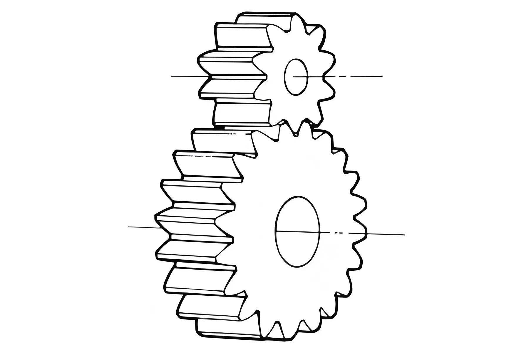
1. Dynamic Model of a Compound-Defect Spur Gear Transmission System
I first constructed a dynamic model that treats the gear pair, flexible shafts, and rolling element bearings as a coupled multi-body system. The model has 36 degrees of freedom and includes the torsional motion of the input and output shafts, the translational motion of the pinion and gear, and the translational motion of the bearing races and resonators. The main assumptions are: (1) pure rolling occurs between the rollers and raceways; (2) elastic deformation in the bearing contacts follows the Hertzian contact theory; (3) manufacturing and mounting errors are neglected; and (4) thermal effects are ignored. These assumptions are acceptable for localized defect diagnosis because the additional displacement caused by a defect is much larger than manufacturing tolerances.
The torsional equation of the input shaft is written as
$$
I_{f1}\ddot{\theta}_{f1} + c_{f1}\bigl(\dot{\theta}_{f1}-\dot{\theta}_{pin}\bigr) + k_{f1}\bigl(\theta_{f1}-\theta_{pin}\bigr) = T_{1}
$$
where \(I_{f1}\) is the input shaft moment of inertia, \(\theta_{f1}\) is the angular displacement of the input shaft, \(c_{f1}\) and \(k_{f1}\) are the torsional damping and stiffness of the input shaft, \(\theta_{pin}\) is the angular displacement of the driving gear, and \(T_1\) is the input torque. Similar equations are written for the output side. For the bearings, the contact forces in the \(x\) and \(y\) directions are
$$
f_{x1} = k_{re1}\sum_{i=1}^{n_b} \gamma_i \delta_i^{n} \cos\theta_i, \qquad
f_{y1} = k_{re1}\sum_{i=1}^{n_b} \gamma_i \delta_i^{n} \sin\theta_i
$$
where \(k_{re1}\) is the equivalent roller-raceway contact stiffness, \(n_b\) is the number of rollers, and the exponent \(n = 1.5\). The parameter \(\gamma_i\) is unity when the local contact deformation \(\delta_i\) is positive, and zero otherwise. The orientation angle of the \(i\)-th roller is
$$
\theta_i = \frac{2\pi(i-1)}{n_b} + \left(1-\frac{d_b}{d_m}\right)\frac{\omega_s}{2}t + \theta_0
$$
where \(d_b\) is the roller diameter, \(d_m\) is the pitch diameter, \(\omega_s\) is the inner ring angular speed, and \(\theta_0\) is the initial cage phase. The contact deformation is
$$
\delta_i = (x_s – x_p)\cos\theta_i + (y_s – y_p)\sin\theta_i – c_o – h_d
$$
in which \(x_s\), \(y_s\), \(x_p\), and \(y_p\) are the displacements of the inner and outer rings, \(c_o\) is the radial clearance, and \(h_d\) is the additional displacement due to a localized defect. For a healthy bearing, \(h_d = 0\).
The nonlinear gear mesh force is defined as
$$
F_M = k_t\bigl(R_{pin}\theta_{pin} – R_{ge}\theta_{ge} – y_{pin} + y_{ge} – \tilde{e}\bigr) + c_t\bigl(R_{pin}\dot{\theta}_{pin} – R_{ge}\dot{\theta}_{ge} – \dot{y}_{pin} + \dot{y}_{ge} – \dot{\tilde{e}}\bigr)
$$
where \(R_{pin}\) and \(R_{ge}\) are the base circle radii, \(y_{pin}\) and \(y_{ge}\) are the translational displacements in the off-line-of-action direction, and \(\tilde{e}\) is the loaded static transmission error. The mesh stiffness \(k_t\) is obtained by combining the bending, shear, radial compression, Hertzian contact, and gear body flexibility stiffnesses. For a tooth with a spalling defect, the cross-sectional area and area moment of inertia are modified, and the bending stiffness becomes
$$
\frac{1}{k_b} = \int_{R_b}^{R_1 – b_s/2} \frac{3\bigl\{1+\cos\alpha_1[(\alpha_2-\alpha)\sin\alpha-\cos\alpha]\bigr\}^2(\alpha_2-\alpha)\cos\alpha}{2 E L [\sin\alpha+(\alpha_2-\alpha)\cos\alpha]^3}\,d\alpha
$$
$$
\quad + \int_{R_1-b_s/2}^{R_1+b_s/2} \frac{12\bigl\{1+\cos\alpha_1[(\alpha_2-\alpha)\sin\alpha-\cos\alpha]\bigr\}^2(\alpha_2-\alpha)\cos\alpha}{E\bigl\{8L[\sin\alpha+(\alpha_2-\alpha)\cos\alpha]^3 – (h_s/R_b)^3 a_s\bigr\}}\,d\alpha
$$
$$
\quad + \int_{R_1+b_s/2}^{R_a} \frac{3\bigl\{1+\cos\alpha_1[(\alpha_2-\alpha)\sin\alpha-\cos\alpha]\bigr\}^2(\alpha_2-\alpha)\cos\alpha}{2 E L [\sin\alpha+(\alpha_2-\alpha)\cos\alpha]^3}\,d\alpha
$$
where \(a_s\), \(b_s\), and \(h_s\) are the spalling length, width, and depth respectively, \(E\) is Young’s modulus, \(L\) is the tooth face width, and \(R_b\), \(R_1\), and \(R_a\) are the base radius, spalling boundary radius, and addendum radius. The shear and radial compression stiffnesses are formulated in the same manner. The bearing localized fault is modeled by an additional displacement \(h_d\). For an outer raceway defect, the additional displacement is active only when the rolling element passes over the defect angular interval, while for an inner raceway defect, the defect position rotates with the shaft.
The key parameters used in the simulation are summarized in Tables 1 and 2. Table 1 gives the main inertia and stiffness parameters of the transmission system, and Table 2 gives the gear pair parameters.
| Parameter | Value |
|---|---|
| Pinion mass \(m_{pin}\) | 0.96 kg |
| Gear mass \(m_{ge}\) | 2.88 kg |
| Pinion moment of inertia \(I_{pin}\) | 4.365e-4 kg·m² |
| Gear moment of inertia \(I_{ge}\) | 8.362e-4 kg·m² |
| Input shaft inertia \(I_{f1}\) | 0.0021 kg·m² |
| Output shaft inertia \(I_{f2}\) | 0.0105 kg·m² |
| Shaft torsional stiffness \(k_{f1}, k_{f2}\) | 4.4e4 N·m/rad |
| Shaft torsional damping \(c_{f1}, c_{f2}\) | 5.0e5 N·m·s/rad |
| Bearing support stiffness \(k_{sj},k_{pj},k_{rj}\) | 6.56e7 N/m |
| Bearing support damping \(c_{sj},c_{pj},c_{rj}\) | 1.8e5 N·s/m |
| Mean transmission error \(e_0\) | 2e-5 m |
| Transmission error amplitude \(e_m\) | 3e-5 m |
| Parameter | Pinion | Gear |
|---|---|---|
| Module \(m\) | 2.5 mm | 2.5 mm |
| Number of teeth \(z\) | 23 | 81 |
| Pressure angle \(\alpha\) | 20° | 20° |
| Face width \(L\) | 26 mm | 26 mm |
| Young’s modulus \(E\) | 206 GPa | 206 GPa |
| Poisson’s ratio \(\nu\) | 0.3 | 0.3 |
The bearing types assigned to the four supports are 6304 for bearings 1 and 2, and 6308 for bearings 3 and 4. These bearings are common deep-groove ball bearings in small and medium gearboxes. In the simulation, the spalling length, width, and depth on the pinion are 6 mm, 0.5 mm, and 0.2 mm respectively. The bearing outer raceway defect length and depth are 0.3556 mm and 0.1794 mm. For the inner raceway defect, the same length and depth are used.
2. Vibration Response Under Variable Operating Conditions
In real applications, the driving motor speed and the load torque are not always constant. External disturbances, control errors, and load variations make the vibration response of a faulted gearbox non-stationary. To study this problem, I solved the dynamic model under four types of conditions: variable speed, variable load, speed fluctuation, and load fluctuation. I processed the bearing housing acceleration with the short-time Fourier transform (STFT) because STFT can represent the time-varying frequency content of non-stationary signals.
When the pinion has a spalling defect and bearing 1 has an outer raceway pitting defect, I set the initial motor speed to 1800 rpm and increased it at a rate of 600 rpm/s for 2 s. The load torque was kept constant at 30 N·m. The time-domain acceleration of the bearing 1 resonator exhibits clear periodic impacts caused by the spalled tooth. As the speed increases, the impact amplitude grows and the time interval between successive impacts decreases. The STFT spectrum contains the gear mesh frequency \(f_m\), the sidebands \(f_m-3f_{r1}\) and \(f_m-4f_{r1}\), and the bearing outer raceway defect frequency \(f_{o1}\). The frequency values increase with speed, but the overall spectral pattern remains similar.
When the inner raceway of bearing 1 has a pitting defect together with the spalled gear, the STFT spectrum in the variable-speed case contains \(f_m\), \(f_m \pm f_{r1}\), \(f_{i1}\), \(f_{i1} \pm f_{r1}\), \(2f_{i1}\), and \(2f_{i1} \pm f_{r1}\). The defect frequency amplitudes increase with speed. I transformed the STFT data into a pseudo-order spectrum by dividing the frequency by the instantaneous shaft rotational frequency \(f_r\). The pseudo-order spectrum is useful when the speed changes because the characteristic orders of the gear and bearing remain constant. The pinion order is 1, the gear mesh order is 23, the bearing outer raceway order is about 2.57, and the inner raceway order is about 4.43. The sideband order families \(3O_i \pm 1\) appear clearly, confirming the presence of an inner raceway defect.
For the variable load condition, I kept the motor speed constant at 1800 rpm and increased the load torque linearly from 15 N·m to 30 N·m over 2 s. The time-domain acceleration amplitude increases with the load, but the characteristic frequencies do not shift. The STFT spectrum shows horizontal lines at \(f_m\), \(2f_m\), and at the bearing defect frequencies; only their amplitudes increase with time. I extracted the amplitude of \(f_{o1}\), \(2f_{o1}\), and \(f_m\), and found a nearly linear increase with load.
I also investigated speed fluctuation and load fluctuation. The actual rotation frequency was expressed as
$$
f = f’ + A\sin(2\pi t + \varphi_1)
$$
where \(f’ = 40\) Hz is the target frequency and \(A = 0.5\) Hz is the fluctuation amplitude. The load torque fluctuation was represented by
$$
T = T’ + B\sin(2\pi t + \varphi_2)
$$
with \(T’ = 30\) N·m and \(B = 10\) N·m. Under speed fluctuation, both the defect frequencies and their amplitudes oscillate with the speed. Under load fluctuation, the defect frequencies remain constant but the amplitudes oscillate with the load. These phenomena are summarized in Table 3.
| Operating condition | Frequency variation | Amplitude variation |
|---|---|---|
| Acceleration | Defect frequencies increase with speed | Amplitudes increase with speed |
| Variable load | Defect frequencies remain constant | Amplitudes increase with load |
| Speed fluctuation | Defect frequencies fluctuate with speed | Amplitudes fluctuate with speed |
| Load fluctuation | Defect frequencies remain constant | Amplitudes fluctuate with load |
The variable-condition analysis clearly indicates that if the rotational speed or load changes during measurement, the spectral amplitudes alone cannot be used directly as a fault severity index. Instead, the instantaneous shaft speed and load must be considered. The STFT and pseudo-order spectra provide reliable tools for tracking the evolution of fault-related components under non-stationary conditions.
3. Coupling Relationship Between Gear Pair and Bearings
In many existing gearbox models, the gear pair and the bearings are treated independently: the bearing is excited by the gear mesh force through the shaft, but the bearing response is not fed back to the gear mesh stiffness. This assumption is not realistic when the shaft is flexible and the bearing clearances are significant. In this work, I introduced a coupling relationship between the gear pair and the bearings through the gyroscopic motion of the transmission shaft. The asynchronous vibration of the bearing inner rings causes the shaft centerline to tilt and translate. As a result, the instantaneous center distance \(a’\) and the misalignment angle \(\theta\) of the gear pair become time-varying.
The geometric relationship is illustrated conceptually by the positions of the bearing inner rings at two axial planes. If the two bearing inner ring displacements are \((x_{s1}, y_{s1})\) and \((x_{s2}, y_{s2})\), and the axial distance between the two bearing centers is \(L\), then the misalignment angle of the shaft axis is
$$
\theta = \arccos\left(\frac{\sqrt{(x_{s2}-x_{s1})^2+(y_{s2}-y_{s1})^2}}{\sqrt{(x_{s2}-x_{s1})^2+(y_{s2}-y_{s1})^2+L^2}}\right)
$$
and the actual center distance projected on the gear plane is
$$
a’ = \sqrt{\left[a – \frac{1}{2}(x_{s1}+x_{s2})\right]^2 + \frac{1}{4}(y_{s1}+y_{s2})^2}
$$
where \(a\) is the theoretical center distance. Since the gear pair is designed for a fixed center distance, any change in \(a’\) changes the operating pressure angle. According to involute gear geometry, the actual pressure angle \(\alpha’\) satisfies
$$
r’ = \frac{r \cos\alpha}{\cos\alpha’}
$$
where \(r\) and \(r’\) are the ideal and actual pitch radii. I used this relation to update the gear mesh stiffness under center distance error and misalignment. In addition, misalignment makes the tooth force distribution non-uniform. The normal load is no longer uniformly distributed along the face width; instead, it is treated as a parabolic distribution with an equivalent torsional component. The potential energy method is extended to derive the bending, shear, radial compression, and torsional stiffness components of a misaligned gear tooth with spalling. The expression for bending stiffness becomes
$$
\frac{1}{k_b} = \int \frac{3\bigl\{1+\cos\alpha_1[(\alpha_2-\alpha)\sin\alpha-\cos\alpha]-f(\alpha,\alpha_1,\alpha_2,\theta)\bigr\}^2(\alpha_2-\alpha)\cos\alpha}{2 E L [\sin\alpha+(\alpha_2-\alpha)\cos\alpha]^3}\,d\alpha
$$
where the function \(f(\alpha,\alpha_1,\alpha_2,\theta)\) includes the effect of the misalignment angle \(\theta\) and the changed lever arm. Similar corrections are applied to the shear stiffness, radial compression stiffness, and torsional stiffness.
I first analyzed a healthy gearbox. Even without faults, the bearing inner ring vibration produces small center distance error and misalignment angle because the gear mesh excitation causes bearing motion. The variation period of these geometrical errors is equal to one mesh cycle, and the resulting mesh stiffness is slightly lower than that of a rigidly supported gear pair. The acceleration response is steady, and the spectrum is dominated by the mesh frequency \(f_m\) and its harmonics \(2f_m\), \(3f_m\). Small sidebands at \(f_m+f_{r1}\) and \(f_m+2f_{r1}\) appear, but their amplitudes are small.
When the pinion has a spalling defect, the mesh stiffness drops inside the defect zone. More importantly, the gear mesh impact causes a sudden change in the bearing displacement, which leads to a sudden change in the center distance and misalignment angle. This geometric disturbance further reduces the mesh stiffness even after the spalled tooth leaves the contact zone, because the shaft gyroscopic motion takes a few vibration cycles to decay. The time-domain acceleration shows an impact at the pinion rotational frequency. The FFT spectrum displays the mesh frequency harmonics and the sidebands \(f_m\pm f_r\) and \(f_m\pm 2f_r\). Interestingly, I also observed the bearing outer raceway defect frequency in the spectrum when the gear pair was the only faulted component. This happens because the gear impact excites the bearing resonance and the bearing defect-related characteristic frequency appears in the envelope spectrum due to the gear-bearing coupling.
When the bearing inner raceway has a localized defect, the rolling elements that pass over the fault produce a periodic displacement pulse. The pulse causes a sudden jump in the center distance and misalignment angle. The gear mesh stiffness is consequently reduced at the bearing fault frequency. The FFT spectrum contains the inner raceway defect frequency \(f_{i1}\), its harmonics, and sidebands \(f_{i1}\pm f_{r1}\), \(2f_{i1}\pm f_{r1}\). At the same time, sidebands around the mesh frequency, such as \(f_m\pm f_{r1}\) and \(f_m\pm 2f_{r1}\), are also visible. These sidebands indicate that the bearing fault modulates the gear mesh stiffness through the coupling relationship. I therefore conclude that in a coupled gear-shaft-bearing system, the presence of a single fault on either the gear or the bearing can generate characteristic frequencies of both components. This must be carefully considered in diagnostic procedures to avoid misclassification.
For the compound fault case with both gear spalling and bearing inner raceway pitting, a single rotation period contains two distinct impact sources. The time-domain waveform clearly separates the gear spalling impact from the bearing fault impact. In the frequency domain, the mesh frequency harmonics remain dominant, but sidebands and defect frequency families of both the gear and bearing coexist. The combined response is more complex, and the overall vibration amplitude is larger than that of each single fault case.
4. Effect of Bearing Fitting Clearance on Spur Gear Transmission Vibration
In practice, a clearance often appears between the bearing outer ring and the bearing housing due to thermal expansion, wear, or improper assembly. When this clearance exists, the outer ring is no longer rigidly supported. Under the dynamic load of the gear pair, the outer ring collides with the housing and generates impact and friction forces. These forces affect the shaft gyroscopic motion, and the gear mesh behavior becomes even more complicated. Therefore, I extended the coupled gear-shaft-bearing model to include the bearing fitting clearance.
In the model, the bearing outer ring support is represented by nonlinear impact elements rather than linear springs. When the relative displacement between the outer ring center and the housing center is smaller than the clearance \(\delta\), the outer ring is free and no contact force is applied. When the radial displacement \(r_p = x_{p1}\cos\beta + y_{p1}\sin\beta\) exceeds the clearance, the normal contact force is calculated by the Hertzian contact model
$$
P_N = \left[\frac{(r_p-\delta)L^2}{0.8 \times 3.83\times 10^{-5}}\right]^{10/9} + c_N \dot{r}_p
$$
where \(L\) is the contact length, \(c_N\) is the contact damping, and \(\beta\) is the contact angular position. The tangential friction force is
$$
P_T = f_c P_N \operatorname{sign}(v_T)
$$
where \(f_c\) is the friction coefficient and \(v_T\) is the relative tangential velocity. The impact forces are projected onto the fixed \(x\) and \(y\) directions, and the linear stiffness and damping of the outer ring support are set to zero when the clearance is active.
I simulated the system with clearance values of 0.01 mm, 0.03 mm, and 0.05 mm in bearing 1 while keeping the gear mesh and bearing raceway parameters unchanged. The time-domain displacement response of the bearing 1 resonator becomes amplitude-modulated by the bearing outer raceway defect frequency. The envelope oscillation becomes more serious as the clearance increases. I extracted the median line of the time-domain response and found that the interval between adjacent envelope peaks is exactly the outer raceway defect period, which confirms that the clearance enhances the amplitude modulation effect of the bearing fault.
The FFT spectrum in the low-frequency band (0-2500 Hz) contains many harmonics of the bearing outer raceway defect frequency, such as \(10f_{o1}\), \(11f_{o1}\), \(12f_{o1}\), and \(18f_{o1}\). These high-order super-harmonics are not visible in the model without clearance. With increasing clearance, even higher-order terms appear. In the high-frequency band (2500-5000 Hz), the spectrum is dominated by the gear mesh frequency harmonics \(4f_m\), \(5f_m\), \(6f_m\), and \(7f_m\), with sidebands at \(4f_m \pm f_{r1}\), \(5f_m \pm f_{r1}\), \(6f_m \pm f_{r1}\), and \(7f_m \pm f_{r1}\). The clearances amplify these sidebands and excite the super-harmonic response of the gear pair.
To explain the generation of super-harmonics, I examined the shaft center trajectory at bearing 1. In the healthy rigid-support case, the shaft orbit is approximately elliptical and confined to a small region. The y-direction displacement is larger than the x-direction displacement because the gear mesh force acts mainly in the off-line-of-action direction. When the outer ring has a fitting clearance, the shaft orbit becomes irregular. The displacement increases in both directions, and the trajectory decays over several oscillations before settling. In the polar coordinate representation, the number of impact peaks within one rotation period increases with clearance. These additional impacts correspond to the impact and rebound cycles of the outer ring on the bearing housing, and each impact excites a new vibration cycle. The multiple decay cycles are the physical reason for the rich super-harmonic frequencies in the spectrum.
I also studied the influence of input speed on the gear-shaft-bearing system with a fixed clearance of 0.02 mm. The RMS and peak-to-peak values of the time-domain response increase with input speed, meaning that the total vibration energy increases. However, the high-order harmonics of the bearing defect frequency and the gear mesh frequency become weaker at higher speeds. The spectrum is increasingly dominated by the fundamental frequencies \(f_m\) and \(f_{o1}\). This indicates that a higher rotating speed suppresses the super-harmonic response and weakens the gear-bearing coupling effect. The system then vibrates primarily at its fundamental frequencies.
These results are important for practical diagnosis because the fitting clearance can significantly alter the spectral signature of a faulted gearbox. If the analyst is not aware of the clearance effect, the rich super-harmonic frequencies might be mistaken for gear tooth faults or bearing raceway faults at different locations. Therefore, before performing fault classification, one should check whether a clearance exists in the bearing-housing interface.
5. Experimental Study and Fault Diagnosis Method
To verify the dynamic models and improve the diagnostic capability for spur gear systems, I performed experiments on a spur gear transmission test rig. The test rig consists of a driving motor, a two-shaft gearbox, a magnetic powder brake for loading, and four accelerometers mounted on the bearing end caps. The input speed was set to 1800 rpm, and the load was 25 N·m. The pinion has 23 teeth, the gear has 81 teeth, and the sampling frequency was 15 kHz. Four sensors provide redundant measurements, so the test system can be used to evaluate the multi-source information fusion method.
I designed ten experimental groups to cover different fault types and fault severities. The faults include gear tooth spalling with three sizes, bearing outer raceway pitting with three sizes, bearing roller cracking with three sizes, and cage fracture with three gap distances. For the gear, the spalling widths and lengths are 1 mm × 7 mm, 2 mm × 13 mm, and 4 mm × 17 mm, all with a depth of 0.5 mm. For the bearing raceway and rollers, the defect cross-sections are 0.2 mm × 0.2 mm, 0.5 mm × 0.5 mm, and 0.8 mm × 0.8 mm. Table 4 summarizes the ten experimental groups and their corresponding labels.
| Experiment | Pinion | Bearing inner race | Roller | Cage | Label |
|---|---|---|---|---|---|
| 1 | Healthy | Healthy | Healthy | Healthy | 1 |
| 2 | Spalling 1×7 | Pitting 0.2×0.2 | Healthy | Healthy | 2 |
| 3 | Spalling 1×7 | Healthy | Pitting 0.2×0.2 | Healthy | 3 |
| 4 | Spalling 1×7 | Healthy | Healthy | Fracture 0.2 | 4 |
| 5 | Spalling 2×13 | Pitting 0.5×0.5 | Healthy | Healthy | 5 |
| 6 | Spalling 2×13 | Healthy | Pitting 0.5×0.5 | Healthy | 6 |
| 7 | Spalling 2×13 | Healthy | Healthy | Fracture 0.5 | 7 |
| 8 | Spalling 4×17 | Pitting 0.8×0.8 | Healthy | Healthy | 8 |
| 9 | Spalling 4×17 | Healthy | Pitting 0.8×0.8 | Healthy | 9 |
| 10 | Spalling 4×17 | Healthy | Healthy | Fracture 0.8 | 10 |
The raw vibration signals contain environmental noise that may reduce the diagnostic accuracy. I used the dual-tree complex wavelet transform (DT-CWT) for signal denoising. The complex wavelet is written as
$$
\varphi(t) = \varphi_h(t) + i\varphi_g(t)
$$
where \(\varphi_h(t)\) and \(\varphi_g(t)\) are two real orthogonal wavelets. The DT-CWT decomposes the signal into real and imaginary trees, which preserves phase information and approximately guarantees shift invariance. I separated the denoising process from the feature learning process so that the network input is as clean as possible.
After denoising, the four channels of vibration data are fused in the data layer. I used the optimal weighting factor (OWF) method. The fused signal is
$$
X = \sum_{i=1}^{n} W_i x_i
$$
where \(x_i\) is the \(i\)-th sensor signal and \(W_i\) is its weight. The weights minimize the total variance
$$
\sigma^2 = \sum_{i=1}^{n} W_i^2 \sigma_i^2
$$
subject to \(\sum W_i = 1\). The optimal weights are
$$
W_i = \frac{1/\sigma_i^2}{\sum_{j=1}^{n} 1/\sigma_j^2}
$$
This method assigns larger weights to channels with smaller noise variance, thus improving the reliability of the fused signal.
I then built a dual-stream convolutional neural network (TSCNN) that simultaneously uses the frequency spectrum and the wavelet time-frequency image. The 1D-CNN branch takes the FFT spectrum as input, while the 2D-CNN branch takes the wavelet time-frequency image as input. The network structures are shown in Table 5. The 1D-CNN has one input layer, two convolution layers, two pooling layers, and a flatten layer. The 2D-CNN has the same number of layers but operates on 64×64 images. Batch normalization is inserted after each pooling layer to accelerate convergence and reduce internal covariate shift.
| Layer | 1D-CNN | 2D-CNN | Activation |
|---|---|---|---|
| Input | 1×433 FFT spectrum | 64×64×3 time-frequency image | — |
| Conv 1 | 1×5 kernel, 6 filters | 5×5 kernel, 6 filters | ReLU |
| Pooling 1 | 1×3 max pool, stride 3 | 2×2 max pool, stride 2 | — |
| BN 1 | 6 channels | 6 channels | — |
| Conv 2 | 1×3 kernel, 16 filters | 5×5 kernel, 16 filters | ReLU |
| Pooling 2 | 1×3 max pool, stride 3 | 2×2 max pool, stride 2 | — |
| BN 2 | 16 channels | 16 channels | — |
| Flatten | 1×752 | 1×1024 | — |
After the flatten layers, the two branches are concatenated to form a 1776-dimensional global feature vector. Two fully connected layers with 120 and 84 neurons are used, followed by a dropout layer with a probability of 0.5 to reduce overfitting. Finally, a support vector machine (SVM) classifier is used instead of a softmax layer. The SVM decision function is
$$
f(x) = \operatorname{sgn}\left[\sum_{n=1}^{e} y_n \lambda_n K(x,x_n) + b\right]
$$
with the Gaussian kernel
$$
K(x,x_n) = \exp\left(-\frac{\|x-x_n\|^2}{2\sigma^2}\right)
$$
I compared four diagnostic models: OWF-1DCNN, OWF-2DCNN, VCR-TSCNN, and OWF-TSCNN. The first two use only one stream of the network; the third uses the variance contribution rate method for signal fusion; the fourth is the proposed model. The training set contains 80% of the collected samples and the test set contains the remaining 20%. Each sample has 1024 data points, corresponding to two rotation periods of the high-speed shaft. The learning rate is 0.001.
Table 6 shows the comparison results after convergence. The OWF-1DCNN model has the shortest training time but the lowest accuracy on both training and test sets. The OWF-2DCNN model achieves better accuracy because the wavelet time-frequency image contains both time-domain and frequency-domain information. The two TSCNN models achieve the highest accuracy. The proposed OWF-TSCNN model reaches 100% accuracy on the training set and 99.83% accuracy on the test set. The loss entropy is very low, and the overfitting rate is close to unity. Compared with the OWF-1DCNN and OWF-2DCNN models, the training time of the OWF-TSCNN model increases by 14.5%-26.6%. The convergence speed is slightly lower than the single-stream models because the total number of parameters is larger. However, the improvement in accuracy and generalization is substantial.
| Model | Training accuracy (%) | Test accuracy (%) | Loss entropy | Overfitting rate | Time (s) |
|---|---|---|---|---|---|
| OWF-1DCNN | 99.65 | 96.83 | 0.0014 | 1.0801 | 218 |
| OWF-2DCNN | 99.86 | 97.41 | 0.00043 | 1.0453 | 234 |
| VCR-TSCNN | 100 | 99.58 | 0.00015 | 1.0022 | 276 |
| OWF-TSCNN | 100 | 99.83 | 0.00016 | 1.0020 | 268 |
I also visualized the extracted features using t-SNE. The OWF-1DCNN and OWF-2DCNN models separate the fault modes only partially, and some sample points remain dispersed. The TSCNN models produce compact clusters with clear boundaries between different labels. This visual result confirms that the dual-stream learning model has stronger feature extraction ability than either single-stream network alone. The confusion matrix of the OWF-TSCNN model on the test set shows that all ten fault classes are classified correctly. In particular, the roller fault, which is difficult to diagnose because the roller slips in the raceway, is also correctly identified. The high generalization ability is mainly due to the multi-source fusion, which suppresses noise, and the dual-stream feature extraction, which preserves both spectral and time-frequency information.
In addition to the fault diagnosis experiments, I carried out experiments to verify the dynamic models. For the variable-speed case, I used an inner raceway-pitted bearing and a spalled gear. The motor speed increased from 2400 rpm to 3000 rpm with a load of 30 N·m. The measured acceleration spectrum contains the gear mesh frequency, the bearing inner raceway defect frequency, and their sidebands. The amplitudes increase with speed, which agrees with the simulation. For the variable-load case, the speed was fixed at 1800 rpm and the load increased from 30 N·m to 40 N·m. The defect frequencies remained constant while the amplitudes increased, again matching the numerical predictions. For the bearing fitting clearance experiment, I used a clearance of 0.02 mm. The measured time-domain response is amplitude-modulated by the bearing outer raceway defect frequency, and the spectrum contains many super-harmonics of both the gear mesh frequency and the bearing defect frequency. The simulated and experimental spectra show the same main components. These experiments validate the accuracy of the dynamic models and the vibration response analysis.
6. Conclusion and Outlook
In this thesis, I investigated the dynamic behavior of spur gear transmission systems with localized defects through analytical modeling, numerical simulation, and experiments. The main conclusions are summarized as follows.
First, a 36-degree-of-freedom compound-defect spur gear transmission model was developed by combining a spalled gear pair and defective rolling bearings. The model captures the non-stationary nature of the vibration response under variable speed and variable load. The STFT spectrum reveals the defect frequencies of the gear pair and bearings together with their modulation sidebands. During acceleration, both the frequencies and amplitudes increase with speed; during load increase, the frequencies remain constant but the amplitudes increase. Speed and load fluctuations cause corresponding fluctuations in the fault frequencies and amplitudes.
Second, the coupling relationship between the gear pair and the bearings was established through the shaft gyroscopic motion. The asynchronous bearing displacements produce time-varying center distance error and misalignment angle, which reduce the gear mesh stiffness. Localized gear or bearing faults cause sudden changes in these geometrical parameters and further degrade the mesh stiffness. The spectral analysis shows that a single fault can produce characteristic frequencies of both the gear and the bearings, which is important for fault diagnosis.
Third, the bearing fitting clearance was introduced into the coupled gear-shaft-bearing model. The clearance generates impact and friction forces between the outer ring and the housing. It significantly increases the time-domain response, enhances the amplitude modulation of the outer raceway defect frequency, and excites high-order super-harmonics of both the gear and the bearing. Higher input speed increases the overall vibration level but suppresses the super-harmonic response, making the fundamental frequencies more dominant.
Fourth, an OWF-TSCNN fault diagnosis method was proposed and verified. The method uses dual-tree complex wavelet denoising, optimal weighting factor multi-sensor fusion, and a dual-stream CNN with SVM classification. Compared with single-stream models, the OWF-TSCNN model has slightly higher computational cost but significantly better accuracy, feature extraction, and generalization. It reaches 100% training accuracy and 99.83% testing accuracy for the ten fault conditions considered. The experiments also validate the dynamic models and demonstrate the practical value of the proposed diagnostic framework.
For future work, I plan to improve the bearing model by considering the cage and roller dynamics in more detail, and to replace the concentrated-mass shaft model with a continuous rotor model that includes bending and gyroscopic effects. I also intend to study the nonlinear dynamics of the spur gear transmission system using phase diagrams, Poincaré maps, and bifurcation analysis. The combination of nonlinear dynamic analysis and deep-learning-based diagnosis may further enhance the robustness of fault detection in spur gears under extremely variable operating conditions.