
In this article, I present a systematic investigation into the tooth root stress characteristics of multi-modulus involute spur gears. The research is driven by the need to understand how varying modulus ratios and displacement coefficients affect the root stress distribution in gear pairs where the driving and driven wheels possess different modules. Throughout the study, I focus on the analytical derivation of stress calculation formulas based on both the plane cross-section method and the broken-line section method, and I verify the theoretical outcomes through finite element simulations. The findings reveal important trends in stress behavior that can aid in the design of high-capacity spur gears.
1. Introduction
Spur gears remain one of the most widely used power transmission components in mechanical systems due to their high efficiency, compact structure, and reliable performance. However, conventional design practice typically assumes equal modules for both gears in a meshing pair. This assumption, while common, is not a necessary condition for correct meshing. The concept of multi-modulus spur gears arises from the understanding that two involute gears can mesh correctly as long as their normal pitches are equal, even if their modules differ. This relaxation of the equality condition opens new possibilities for gear design optimization, particularly in terms of stress reduction and load-sharing improvement.
The tooth root stress is widely recognized as a primary factor contributing to tooth breakage in spur gears. Therefore, accurate estimation of root stress is essential for ensuring the reliability and durability of gear transmissions. Traditional methods, such as the Lewis formula and the ISO standard, calculate root stress based on a simplified plane cross-section assumption. However, actual gear cracks often propagate along paths that are better represented by a broken-line cross-section. The broken-line section method offers a more realistic assessment by considering the actual transition curve geometry of the gear tooth.
In this research, I aim to bridge the gap in knowledge regarding the tooth root stress behavior of multi-modulus spur gears. I systematically derive the formulas needed to calculate the root stress using both the plane cross-section method and the broken-line section method, adapted specifically for multi-modulus gear pairs. I then analyze how the modulus ratio and displacement coefficients influence the peak root stress and stress distribution along the transition curve. To validate the theoretical calculations, I create accurate three-dimensional models of the gears with precisely generated transition curves and perform finite element simulations. The combination of analytical and computational approaches provides a comprehensive understanding of the stress characteristics in these advanced gear systems.
2. Parameter Calculation for Multi-Modulus Involute Spur Gears
The design and analysis of multi-modulus spur gears require the derivation of meshing parameters and geometric quantities that differ from those of conventional equal-modulus gears. In this section, I present the necessary formulas and constraints that govern the selection of key parameters.
2.1 Correct Meshing Condition
For a pair of involute spur gears to mesh correctly, the normal pitches of the two gears must be equal. For a multi-modulus gear pair, this condition is expressed as:
$$m_p \cos \alpha_p = m_g \cos \alpha_g$$
where mp and mg are the modules of the driving and driven gears, respectively, and αp and αg are the corresponding pressure angles at the pitch circles. The modulus ratio is defined as δm = mp / mg. When the modulus ratio deviates from unity, the pressure angles must adjust accordingly to maintain meshing.
2.2 Meshing Angle and Center Distance
For correct meshing without backlash, the working pitch circle tooth thicknesses of the two gears must sum to the circular pitch. This leads to the following expression for the operating pressure angle (meshing angle) αv:
$$\operatorname{inv} \alpha_v = \frac{x_p + x_g}{z_p + z_g} + \frac{z_p \operatorname{inv} \alpha_p + z_g \operatorname{inv} \alpha_g}{z_p + z_g}$$
where xp and xg are the displacement coefficients, zp and zg are the tooth numbers, and inv denotes the involute function. The actual center distance a1 is given by:
$$a_1 = \frac{m_p z_p \cos \alpha_p + m_g z_g \cos \alpha_g}{2 \cos \alpha_v}$$
2.3 Top Clearance Coefficient and Addendum Coefficient
To ensure proper clearance between the tooth tip of one gear and the tooth root of the other, the clearance coefficients of the two gears must satisfy:
$$c_1^* m_p = c_2^* m_g$$
Similarly, the addendum coefficients are related by:
$$h_{a1}^* m_p = h_{a2}^* m_g$$
From these relationships, it follows that when the modulus ratio δm is greater than unity, the clearance coefficient and addendum coefficient of the driving gear are reduced proportionally.
2.4 Center Distance Modification Coefficient
The center distance modification coefficients y1 and y2 for the driving and driven gears are defined as:
$$y_1 = \frac{a_1 – a}{m_p}, \quad y_2 = \frac{a_1 – a}{m_g}$$
where a is the standard center distance. The addendum reduction coefficients Δy1 and Δy2 are then:
$$\Delta y_1 = x_{\Sigma} – y_1, \quad \Delta y_2 = x_{\Sigma} – y_2$$
where xΣ = xp + xg.
2.5 Constraints on Displacement Coefficients
When analyzing the tooth root stress characteristics of multi-modulus spur gears, the displacement coefficients must be selected within permissible ranges. I consider three primary constraints:
Contact ratio constraint: The contact ratio ε must be greater than 1.2 to ensure smooth transmission:
$$\varepsilon = \frac{m_p z_p (\tan \alpha_{a}^{p} – \tan \alpha_v) + m_g z_g (\tan \alpha_{a}^{g} – \tan \alpha_v)}{2 \pi m_g \cos \alpha_g} > 1.2$$
Tooth tip thickness constraint: The tooth tip thickness must be greater than 0.25 times the module:
$$S_{a1} = d_{a1} \left( \frac{\pi}{2 z_p} + \frac{2 x_p \tan \alpha_p}{z_p} – \operatorname{inv} \alpha_{a}^{p} + \operatorname{inv} \alpha_p \right) > 0.25 m_p$$
Non-interference constraint: The gears must not interfere during meshing, which imposes limits on the combination of modulus ratio and displacement coefficients.
2.6 Constraint on Face Width
The face width of the gears must be large enough to satisfy the bending strength requirement. The condition is given by:
$$b \geq \frac{F_t \; Y_F \; Y_S \; K_A \; K_V \; K_{F\beta} \; K_{F\alpha}}{m \; \sigma_{FP}}$$
where Ft is the tangential force, YF is the form factor, YS is the stress correction factor, and the K terms are various application and load distribution factors.
3. Calculation Methods for Tooth Root Stress
In this section, I describe the two analytical methods I used to calculate the tooth root stress of multi-modulus spur gears: the plane cross-section method and the broken-line section method.
3.1 Plane Cross-Section Method
The plane cross-section method, based on the ISO standard, treats the critical section of the gear tooth as a plane perpendicular to the tooth symmetry axis. The 30° tangent method is used to determine the location of the critical section. The nominal root stress is calculated as:
$$\sigma_{F0} = \frac{F_t}{b m} Y_F Y_S Y_{\beta}$$
where YF is the tooth form factor, YS is the stress correction factor, and Yβ is the helix angle factor (equal to unity for spur gears). The form factor is:
$$Y_F = \frac{6 \left( \frac{h_F}{m} \right) \cos \alpha_F}{\left( \frac{S_F}{m} \right)^2 \cos \alpha}$$
where hF is the bending moment arm, SF is the tooth thickness at the critical section, and αF is the load angle. The stress correction factor is given by:
$$Y_S = \left( 1.2 + 0.13 \frac{S_F}{h_F} \right) \left( \frac{S_F}{2 \rho_e} \right)^{0.13 + 0.21 / \left( \frac{S_F}{h_F} \right)}$$
For multi-modulus spur gears, the formulas are applied separately to the driving and driven gears, incorporating the respective modules and tooth parameters. The final stress is:
$$\sigma_F = \sigma_{F0} K_A K_V K_{F\beta} K_{F\alpha}$$
3.2 Broken-Line Section Method
The broken-line section method recognizes that the critical section of the gear tooth is not a single plane but a broken line perpendicular to the transition curve. This aligns better with the actual crack propagation path observed in practice. The stress at any point on the transition curve is calculated using the local stress coefficient approach.
The transition curve of the gear tooth is generated by the tool tip radius during the hobbing process. Using the principle of gearing, the coordinates of any point on the transition curve can be expressed as:
$$x = (r \varphi – x_1) \cos \varphi + (r – y_1) \sin \varphi$$
$$y = (r \varphi – x_1) \sin \varphi – (r – y_1) \cos \varphi$$
where r is the pitch circle radius, φ is the rolling angle, and (x1, y1) are the coordinates of the tool tip point. For multi-modulus spur gears, the transition curve equations for the driving and driven gears are derived separately with their respective module values.
The tooth root stress at a point on the transition curve is given by:
$$\sigma = \frac{T}{b r m} Y_{\sigma}$$
where T is the input torque and Yσ is the local stress concentration factor:
$$Y_{\sigma} = \frac{2 \cos \alpha}{\left( \frac{Y}{m} \right)^2 \left( \frac{\overline{GD}}{Y} – 2 \cos \delta \sin \delta \tan \psi \right)}$$
In this expression, Y is half the tooth thickness at the point of interest, ψ is the tangent angle, δ is the angle between the load line and the perpendicular to the tooth symmetry axis, and \(\overline{GD}\) is the distance between the intersection of the load line with the axis and the intersection of the normal to the transition curve with the axis.
3.3 Comparison of the Two Methods
The plane cross-section method is widely used due to its simplicity and long history, but it only provides a single stress value at the 30° tangent point and may not capture the true peak stress. In contrast, the broken-line section method yields the stress distribution along the entire transition curve, allowing for the identification of the actual peak stress and its position. The broken-line method is more sensitive to changes in tooth profile parameters, which makes it particularly suitable for analyzing multi-modulus spur gears.
4. Analysis of Tooth Root Stress Characteristics
4.1 Case Study Parameters
To investigate the effects of modulus ratio and displacement coefficients on the tooth root stress characteristics, I selected a gear pair with the basic parameters listed in Table 1. The module of the driven gear is kept constant at mg = 1.25 mm, the pressure angle is 20°, the clearance coefficient is 0.25, and the addendum coefficient is 1.0. The modulus ratio varies from 0.98 to 1.08. The face width is 16 mm, and the input power is 1.64 kW at 1750 r/min.
| No. | mp (mm) | αp (°) | mg (mm) | αg (°) | δm |
|---|---|---|---|---|---|
| 1 | 1.2250 | 16.49 | 1.25 | 20 | 0.98 |
| 2 | 1.2375 | 18.34 | 1.25 | 20 | 0.99 |
| 3 | 1.2500 | 20.00 | 1.25 | 20 | 1.00 |
| 4 | 1.2625 | 21.50 | 1.25 | 20 | 1.01 |
| 5 | 1.2750 | 22.89 | 1.25 | 20 | 1.02 |
| 6 | 1.2875 | 24.17 | 1.25 | 20 | 1.03 |
| 7 | 1.3000 | 25.37 | 1.25 | 20 | 1.04 |
| 8 | 1.3125 | 26.50 | 1.25 | 20 | 1.05 |
| 9 | 1.3250 | 27.56 | 1.25 | 20 | 1.06 |
| 10 | 1.3375 | 28.57 | 1.25 | 20 | 1.07 |
| 11 | 1.3500 | 29.53 | 1.25 | 20 | 1.08 |
4.2 Results from the Plane Cross-Section Method
Using the plane cross-section method, I calculated the peak root stresses for various combinations of modulus ratio and displacement coefficients. Table 2 shows the driving gear root stress as functions of modulus ratio and driving gear displacement coefficient.
| δm | xp = -0.3 | xp = -0.2 | xp = -0.1 | xp = 0 | xp = 0.1 | xp = 0.2 | xp = 0.3 |
|---|---|---|---|---|---|---|---|
| 0.98 | 219.2 | 206.6 | 196.9 | 189.4 | 183.8 | 179.7 | 176.8 |
| 1.00 | 180.7 | 173.5 | 168.0 | 164.0 | 161.1 | 159.1 | 157.8 |
| 1.02 | 156.6 | 152.5 | 149.4 | 147.1 | 145.7 | 144.8 | 144.4 |
| 1.04 | 140.6 | 138.1 | 136.3 | 135.2 | 134.5 | 134.4 | 134.3 |
| 1.06 | 129.3 | 127.8 | 126.8 | 126.2 | 126.0 | 126.1 | 126.4 |
The results indicate that for modulus ratios between 0.98 and 1.04, the driving gear root stress decreases monotonically with increasing displacement coefficient. However, at δm = 1.05 and 1.06, a slight non-monotonic trend is observed, which is attributed to the shifting of the peak stress location away from the 30° tangent point.
4.3 Results from the Broken-Line Section Method
With the broken-line section method, I obtained the full stress distribution along the transition curve. This allows for a more accurate determination of the peak stress. Figure 1 illustrates the distribution of the tooth root stress along the transition curve for the driving gear under different modulus ratios.
The stress distribution curves exhibit a clear trend: the stress increases as the tangent angle increases from the root to a maximum value near 30°, then decreases toward the involute portion. This confirms that the maximum stress occurs around a 30° tangent angle, consistent with observations in conventional spur gears. The specific location of the peak shifts slightly with changes in the modulus ratio and displacement coefficient.
Tables 3 and 4 summarize the peak stress values obtained from the broken-line section method for the driving and driven gears, respectively, under various combinations of modulus ratio and driving gear displacement coefficient.
| δm | xp = -0.3 | xp = -0.2 | xp = -0.1 | xp = 0 | xp = 0.1 | xp = 0.2 | xp = 0.3 |
|---|---|---|---|---|---|---|---|
| 0.98 | 151.0 | 140.1 | 131.8 | 125.7 | 121.1 | 117.8 | 115.7 |
| 1.00 | 121.9 | 115.7 | 111.0 | 107.5 | 105.0 | 103.3 | 102.2 |
| 1.02 | 105.0 | 101.1 | 98.2 | 96.1 | 94.6 | 93.7 | 93.2 |
| 1.04 | 94.1 | 91.6 | 89.7 | 88.3 | 87.4 | 86.8 | 86.7 |
| 1.06 | 86.8 | 85.0 | 83.6 | 82.7 | 82.1 | 81.8 | 81.7 |
| δm | xp = -0.3 | xp = -0.2 | xp = -0.1 | xp = 0 | xp = 0.1 | xp = 0.2 | xp = 0.3 |
|---|---|---|---|---|---|---|---|
| 0.98 | 92.4 | 94.9 | 97.2 | 99.5 | 101.6 | 103.7 | 105.7 |
| 1.00 | 96.1 | 98.8 | 101.4 | 103.9 | 106.3 | 108.6 | 110.8 |
| 1.02 | 100.4 | 103.3 | 106.0 | 108.6 | 111.1 | 113.6 | 116.0 |
| 1.04 | 105.0 | 107.9 | 110.8 | 113.5 | 116.1 | 118.7 | 121.1 |
| 1.06 | 109.8 | 112.8 | 115.6 | 118.4 | 121.1 | 123.7 | 126.3 |
From the broken-line section method results, it is evident that:
- For a fixed modulus ratio, the driving gear peak root stress decreases with increasing displacement coefficient, while the driven gear peak root stress increases.
- For a fixed displacement coefficient, both gears exhibit monotonic trends: the driving gear stress decreases with increasing modulus ratio, whereas the driven gear stress increases.
- The modulus ratio has a more pronounced effect on the peak stress compared to the displacement coefficient.
4.4 Tangent Angle at Peak Stress
One important finding of this study is that the tangent angle corresponding to the peak root stress is not always exactly 30°. It varies with the modulus ratio and displacement coefficients. Tables 5 and 6 show the tangent angles at which the peak stress occurs for the driving and driven gears under different parameter combinations.
| δm | xp = -0.3 | xp = -0.2 | xp = -0.1 | xp = 0 | xp = 0.1 | xp = 0.2 | xp = 0.3 |
|---|---|---|---|---|---|---|---|
| 0.98 | 22.61 | 23.96 | 25.72 | 26.57 | 27.46 | 28.01 | 28.30 |
| 1.00 | 24.75 | 25.77 | 27.32 | 28.18 | 28.90 | 28.99 | 29.41 |
| 1.02 | 27.38 | 28.19 | 28.85 | 29.33 | 29.58 | 29.72 | 29.73 |
| 1.04 | 28.49 | 29.06 | 29.63 | 30.00 | 30.08 | 30.01 | 29.72 |
| 1.06 | 29.31 | 29.79 | 30.05 | 30.23 | 30.31 | 30.24 | 29.90 |
In Table 5, for δm between 0.98 and 1.03, the tangent angle at peak stress is consistently below 30° and increases with increasing displacement coefficient. For δm between 1.04 and 1.06, the tangent angle first increases beyond 30° and then decreases, causing the non-monotonic behavior observed in the plane-cross-section results.
5. Three-Dimensional Modeling and Finite Element Simulation
5.1 Model Generation for Multi-Modulus Spur Gears
To validate the theoretical findings, I developed accurate three-dimensional solid models of the multi-modulus spur gears. The transition curve of the gear tooth profile is the most critical part for accurate stress analysis. I generated the transition curve data points using MATLAB based on the derived transition curve equations, and then imported these data points into SolidWorks to create the precise tooth profile geometry.
The modeling procedure consists of the following steps:
- Calculate all gear parameters using the formulas derived in Section 2.
- Generate the transition curve coordinates using MATLAB for the specific modulus ratio and displacement coefficient.
- Import the coordinate data into SolidWorks and fit a spline curve through the points.
- Construct the complete tooth profile by combining the transition curve, involute curve, tip circle, and root circle.
- Create the three-dimensional gear model by extruding and patterning the tooth profile.
- Assemble the driving and driven gears at the calculated center distance.
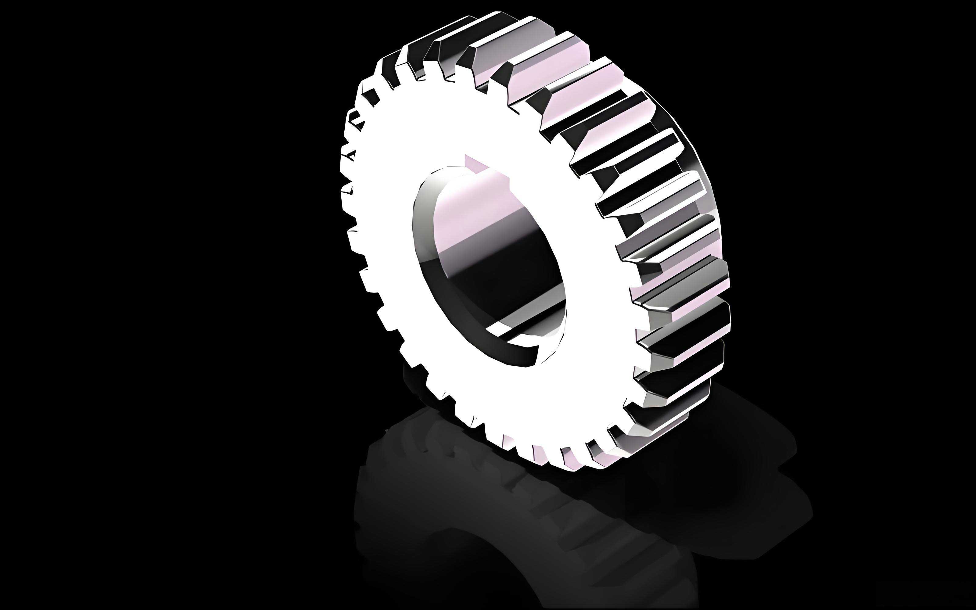
The assembled gear pair model for δm = 1.02 is shown in the figure below. This model was used for all subsequent finite element simulations.
5.2 Finite Element Simulation Setup
For the finite element analysis, I performed static structural simulations. The boundary conditions included a clockwise driving torque of 8949 N·mm applied to the driving gear, while the driven gear was fully constrained. The gears were meshed with tetrahedral elements, with a global element size of 0.5 mm and a refined mesh of 0.1 mm on the tooth root transition surfaces where stress was to be evaluated.
The contact at the meshing point was modeled as frictional contact with a friction coefficient of 0.2. The material was set to structural steel with default properties, as the study focuses on geometric influences rather than material-specific behavior.
5.3 Simulation Results
The finite element analysis yielded the equivalent stress distribution on the gear teeth. The stress distribution along the transition curve showed a clear pattern: the stress increases from the root toward the middle of the transition region, reaches a maximum near the 30° tangent point, and then decreases toward the start of the involute profile. This behavior is consistent with the analytical predictions from the broken-line section method.
Tables 7 and 8 present the peak root stress values obtained from the finite element simulations for the driving and driven gears, respectively.
| δm | xp = -0.3 | xp = -0.2 | xp = -0.1 | xp = 0 | xp = 0.1 | xp = 0.2 | xp = 0.3 |
|---|---|---|---|---|---|---|---|
| 0.98 | 148.07 | 140.41 | 132.36 | 124.94 | 120.06 | 116.33 | 115.49 |
| 1.00 | 123.23 | 117.43 | 111.55 | 110.27 | 109.62 | 105.61 | 101.40 |
| 1.02 | 107.25 | 102.15 | 100.84 | 100.07 | 95.31 | 94.17 | 94.07 |
| 1.04 | 96.28 | 95.77 | 95.32 | 95.05 | 94.01 | 92.65 | 89.70 |
| 1.06 | 94.69 | 93.15 | 90.21 | 89.92 | 88.46 | 86.75 | 84.03 |
| δm | xp = -0.3 | xp = -0.2 | xp = -0.1 | xp = 0 | xp = 0.1 | xp = 0.2 | xp = 0.3 |
|---|---|---|---|---|---|---|---|
| 0.98 | 89.66 | 91.63 | 99.82 | 100.27 | 102.20 | 118.40 | 118.70 |
| 1.00 | 98.68 | 99.90 | 102.42 | 105.43 | 121.17 | 122.29 | 123.28 |
| 1.02 | 113.26 | 113.98 | 118.52 | 120.91 | 121.59 | 122.97 | 134.44 |
| 1.04 | 113.72 | 117.09 | 120.20 | 121.84 | 122.66 | 128.79 | 136.08 |
| 1.06 | 118.01 | 120.62 | 122.28 | 130.68 | 133.98 | 135.90 | 137.75 |
5.4 Comparison of FEM and Analytical Results
Comparing the finite element results with the analytical calculations reveals the following:
- The stress distribution along the transition curve obtained from FEM exactly matches the broken-line section method results.
- The variation trends of the peak root stress with respect to the modulus ratio and displacement coefficient are consistent between FEM and the broken-line section method.
- The numerical values from the broken-line section method are much closer to the FEM results than those from the plane cross-section method.
Table 9 shows the differences between FEM results and the broken-line section method predictions for the driving gear root stress. The maximum difference is 8.41 MPa, corresponding to a percentage error of approximately 8.8%. Table 10 shows the corresponding differences between FEM and the plane cross-section method, where the minimum difference is 34.6 MPa, corresponding to an error of approximately 36.6%.
| δm | xp = -0.3 | xp = -0.2 | xp = -0.1 | xp = 0 | xp = 0.1 | xp = 0.2 | xp = 0.3 |
|---|---|---|---|---|---|---|---|
| 0.98 | 2.93 | -0.31 | -0.56 | 0.76 | 1.04 | 1.47 | 0.21 |
| 1.00 | -1.33 | -1.73 | -0.55 | -2.77 | -4.62 | -2.31 | 0.80 |
| 1.02 | -2.25 | -1.05 | -2.60 | -3.98 | -0.71 | -0.51 | -0.87 |
| 1.04 | -2.15 | -4.18 | -5.65 | -6.77 | -6.65 | -5.81 | -3.04 |
| 1.06 | -7.91 | -8.17 | -6.59 | -7.25 | -6.41 | -5.00 | -2.32 |
| δm | xp = -0.3 | xp = -0.2 | xp = -0.1 | xp = 0 | xp = 0.1 | xp = 0.2 | xp = 0.3 |
|---|---|---|---|---|---|---|---|
| 0.98 | 71.13 | 66.19 | 64.54 | 64.46 | 63.74 | 63.37 | 61.31 |
| 1.00 | 57.47 | 56.07 | 56.45 | 53.73 | 51.48 | 53.49 | 56.40 |
| 1.02 | 49.35 | 50.35 | 48.56 | 47.03 | 50.39 | 50.63 | 50.33 |
| 1.04 | 44.32 | 42.33 | 40.98 | 40.15 | 40.50 | 41.75 | 44.65 |
| 1.06 | 34.61 | 34.65 | 36.59 | 36.28 | 37.54 | 39.35 | 42.37 |
These comparisons clearly demonstrate that the broken-line section method provides significantly more accurate predictions for the tooth root stress in multi-modulus spur gears compared to the conventional plane cross-section method. The small remaining discrepancies between FEM and the broken-line method can be attributed to mesh discretization, contact modeling approximations, and minor geometric simplifications.
6. Summary and Conclusions
In this research, I conducted a comprehensive analysis of the tooth root stress characteristics of multi-modulus involute spur gears. The key contributions and findings of this work are summarized as follows:
-
I derived the meshing parameter formulas for multi-modulus spur gears, including the operating pressure angle, center distance, clearance coefficient, addendum coefficient, and center distance modification coefficients. These formulas account for the unequal modules of the two gears and ensure proper meshing conditions.
-
I established the allowable ranges for displacement coefficients under different modulus ratios by considering the contact ratio, tooth tip thickness, and non-interference constraints. These constraints are essential for ensuring that the designed gears can operate reliably.
-
I adapted both the plane cross-section method and the broken-line section method to calculate the tooth root stress of multi-modulus spur gears. The broken-line section method, in particular, can provide the full stress distribution along the transition curve and identify the actual peak stress location.
-
Through extensive parametric studies, I identified the following stress characteristics:
- The driving gear root stress decreases with increasing modulus ratio, while the driven gear stress increases.
- Increasing the driving gear displacement coefficient reduces the driving gear stress but increases the driven gear stress.
- Increasing the driven gear displacement coefficient has the opposite effect: it reduces the driven gear stress but increases the driving gear stress.
- The modulus ratio has a more significant influence on the root stress than the displacement coefficients in the studied ranges.
-
The peak stress location is not always at the 30° tangent point. It shifts slightly with changes in modulus ratio and displacement coefficients, which can cause discrepancies between the plane cross-section method and the actual stress.
-
I created accurate three-dimensional models of multi-modulus spur gears with precisely generated transition curves and verified the analytical results through finite element simulations. The simulation results confirm that the broken-line section method yields stress values that are in much better agreement with FEM results (errors within 8.8%) compared to the plane cross-section method (errors of 36% or more).
These findings provide a solid theoretical foundation for the design and optimization of multi-modulus spur gears, helping to improve their load-carrying capacity and reliability. Future work could extend this analysis to consider tooth profile modifications, dynamic loading conditions, and the influence of additional geometric parameters such as tooth number ratios.