
Spur gears are the core transmission elements used across modern industrial equipment, from automotive gearboxes to heavy machinery. Their reliable operation is critical because unexpected gear failures can cause significant production losses and severe safety accidents. In this research, I focus on the early fault diagnosis of spur gears under non-stationary running conditions by analyzing vibration signals. The complexity of vibration signals collected from a spur gearbox is high, because the measured waveforms contain not only gear meshing components but also noise and interference from adjacent rotational components. I therefore investigate an integrated method combining enhanced signal decomposition, refined feature extraction, and optimized support vector machines, so that weak early-stage faults in a spur gear can be detected with high accuracy.
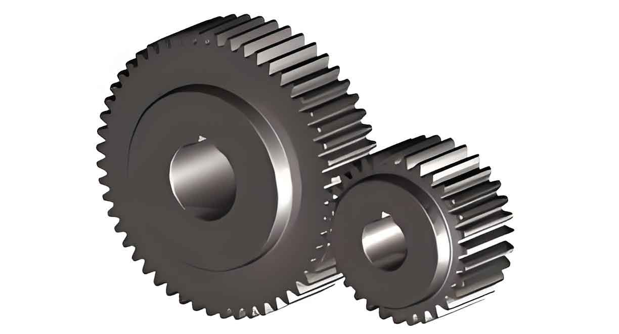
In my study, the main contributions are as follows. First, I establish a dynamic model of a spur gear pair and analyze the modulation sidebands caused by distributed and localized gear faults. Second, I propose a signal preprocessing framework that uses singular value kurtosis difference spectrum to determine the optimal decomposition level in variational mode decomposition, and then combines optimized maximum correlated kurtosis deconvolution to enhance weak pulse features. Third, I extract multi-domain features from the processed vibration signals, select the most informative features with random forest, and fuse them using principal component analysis. Finally, I construct a hybrid kernel support vector machine model whose penalty parameter, kernel width, and kernel weight are optimized by the dung beetle optimizer. The proposed method is verified on a self-built spur gear fault diagnosis experimental platform, and the results show that it can reliably distinguish healthy gears, worn gears, pitted gears, broken-tooth gears, and compound faults.
1. Background and Significance of Spur Gear Fault Diagnosis
With the rapid development of intelligent manufacturing, traditional mechanical equipment is moving toward digitization and automation. Spur gears are widely used in transmission systems because of their simple structure, high transmission efficiency, and stable operation. However, because spur gear teeth repeatedly engage and disengage under heavy loads, they are vulnerable to fatigue damage. Typical damage modes include tooth breakage, surface pitting, and tooth wear. In many industrial cases, a spur gear fault develops gradually, and if it is not detected in time, it may lead to machine breakdown. Therefore, online condition monitoring and early fault diagnosis of spur gears play a vital role in reducing maintenance costs and improving system safety.
Vibration-based diagnosis is one of the most effective techniques for spur gear health monitoring. When a fault occurs in a spur gear, the stiffness and load distribution change, which causes amplitude and frequency modulation in the measured vibration signal. These modulations produce sidebands around the gear meshing frequency and its harmonics. Extracting these sidebands from a noisy signal, especially under non-stationary operating conditions, remains a significant challenge. Early fault symptoms are often weak, and the period impulses are covered by strong background noise. Hence, robust signal decomposition and feature enhancement methods are needed.
2. Vibration Mechanism and Signal Characteristics of Spur Gear
The vibration of a spur gear pair is generated by time-varying mesh stiffness and dynamic excitation. In my research, I first build a simplified dynamic model of the spur gear pair. The gear pair can be represented as two inertias connected by a spring and damper at the mesh point.
$$M_m \ddot{x} + C \dot{x} + K(t)x = F(t)$$
where $M_m$ is the equivalent mass of the spur gear pair, $C$ is the mesh damping, $K(t)$ is the time-varying mesh stiffness, $x$ is the relative displacement along the line of action, and $F(t)$ is the dynamic excitation force. The mesh stiffness $K(t)$ changes periodically because the number of teeth in contact alternates between one pair and two pairs. This periodic stiffness variation is one of the main internal excitations of spur gear vibration.
In order to analyze the tooth bending, shear, and contact deformation, I model the spur gear tooth as a variable-section cantilever beam. The total mesh stiffness of a single tooth pair can be expressed as:
$$\frac{1}{k_m} = \sum_{i=1}^{2} \left( \frac{1}{k_{b,i}} + \frac{1}{k_{s,i}} + \frac{1}{k_{a,i}} + \frac{1}{k_{f,i}} + \frac{1}{k_{e,i}} \right) + \frac{1}{k_{h}}$$
where $k_{b,i}$ is the bending stiffness, $k_{s,i}$ is the shear stiffness, $k_{a,i}$ is the axial compressive stiffness, $k_{f,i}$ is the fillet foundation stiffness, $k_{e,i}$ is the gear body flexibility, and $k_h$ is the Hertzian contact stiffness. The subscripts 1 and 2 represent the driving and driven spur gear, respectively. In a healthy spur gear, the mesh stiffness fluctuates at the gear mesh frequency $f_m$, which is determined by the shaft rotational frequency and the number of teeth:
$$f_m = N_1 f_{r1} = N_2 f_{r2}$$
where $N_1$ and $N_2$ are the numbers of teeth of the driving and driven gears, and $f_{r1}$ and $f_{r2}$ are the corresponding shaft rotation frequencies. In the actual measurement, the spur gear vibration signal contains the meshing frequency, its harmonics, sidebands, shaft-related frequency components, and a large amount of background noise.
To describe the measured vibration signal of a faulty spur gear, I use a modulation model:
$$x(t) = \sum_{i=1}^{n} X_i \left[ 1 + a_i(t) \right] \cos \left[ 2\pi i f_m t + \varphi_i + b_i(t) \right]$$
where $X_i$ is the amplitude of the $i$-th harmonic, $a_i(t)$ is the amplitude modulation function, $b_i(t)$ is the frequency modulation function, and $\varphi_i$ is the initial phase. When a spur gear tooth has a local defect, the defect produces a short impact once per revolution, which appears in the vibration signal as amplitude modulation. When the gear is eccentric or has non-uniform tooth spacing, frequency modulation occurs. In most actual cases, amplitude and frequency modulation coexist, generating asymmetric sidebands around the meshing harmonics.
The typical spur gear fault modes and their occurrence proportions are summarized below.
| Fault mode | Occurrence ratio | Typical symptom in vibration spectrum |
|---|---|---|
| Tooth breakage | 41% | Large periodic impulses; dense sideband clusters around mesh frequency |
| Tooth surface pitting | 31% | Extra spectral peaks; broad energy around mesh frequency and harmonics |
| Tooth wear and scuffing | 20% | Increased noise level; sidebands with irregular spacing |
| Other faults | 8% | Combination of the above patterns |
3. Vibration Signal Processing Based on Improved VMD and MCKD
In a non-stationary spur gear system, the acquired vibration signal is usually contaminated by environmental noise and vibrations from bearings and shafts. Directly extracting fault features from the raw signal is difficult. In my method, I first use variational mode decomposition to decompose the signal into a set of band-limited intrinsic mode functions. VMD is a fully non-recursive decomposition algorithm, which determines the central frequency and bandwidth of each mode by solving an optimization problem. The constrained variational model for a spur gear vibration signal $f(t)$ is written as:
$$\min_{\{u_k\}, \{\omega_k\}} \left\{ \sum_{k=1}^{K} \left\| \partial_t \left[ \left( \delta(t) + \frac{j}{\pi t} \right) * u_k(t) \right] e^{-j \omega_k t} \right\|_2^2 \right\} \quad \text{s.t.} \quad \sum_{k=1}^{K} u_k(t) = f(t)$$
where $u_k(t)$ is the $k$-th intrinsic mode function, $\omega_k$ is its center frequency, $K$ is the number of modes, and $\delta(t)$ is the Dirac delta function. To solve this constrained optimization problem, I introduce the quadratic penalty parameter $\alpha$ and the Lagrangian multiplier $\lambda(t)$, then use the alternating direction method of multipliers to update the modes, center frequencies, and multipliers iteratively.
3.1 Determination of Optimal Decomposition Level
Choosing the correct number of modes $K$ is a key issue. If $K$ is too small, the decomposed modes will mix together; if $K$ is too large, over-decomposition occurs. In my method, I propose to use the singular value kurtosis difference spectrum to set the initial $K$. First, the Hankel matrix of the raw signal is constructed and singular value decomposition is performed:
$$D = U \Sigma V^T$$
where $U$ and $V$ are orthogonal matrices and $\Sigma$ is a diagonal matrix containing the singular values. The difference between neighboring singular values is defined as:
$$b_i = \sigma_i – \sigma_{i+1}, \quad i = 1, 2, \ldots, n-1$$
The sequence $b_i$ is called the singular value difference spectrum. A sharp peak in this difference spectrum indicates the boundary between the dominant signal component and noise. Since the kurtosis is sensitive to impact components in a spur gear signal, I calculate the kurtosis of the singular value sequence and locate the maximum kurtosis peak in the difference spectrum. The corresponding index is used as the initial decomposition level $K_0$. Then, after performing VMD with $K_0$, I check whether two adjacent modes have center frequencies too close to each other:
$$\frac{|\omega_i – \omega_{i+1}|}{(\omega_i + \omega_{i+1})/2} \le \delta$$
where $\delta$ is set to 0.1. If this condition is satisfied, the modes are considered to be over-split, and the decomposition number is reduced by one. The process is repeated until no over-decomposition is detected, giving the final optimal $K$.
3.2 IMF Selection and Signal Reconstruction
After VMD decomposition, I need to choose the modes that contain useful fault information. I calculate the correlation coefficient $r_{xy}$ between each intrinsic mode function and the original spur gear vibration signal:
$$r_{xy} = \frac{\sum_{i=1}^{N} (x_i – \bar{x})(y_i – \bar{y})}{\sqrt{\sum_{i=1}^{N} (x_i – \bar{x})^2 \sum_{i=1}^{N} (y_i – \bar{y})^2}}$$
I also calculate the kurtosis value of each mode:
$$k = \frac{\mathbb{E} \left[ (x(t) – \mu)^4 \right]}{\sigma^4}$$
where $\mu$ is the mean and $\sigma$ is the standard deviation. A healthy vibration signal usually has a kurtosis close to 3, while a faulty spur gear signal has a larger kurtosis. In my selection rule, a mode is retained when its correlation coefficient is larger than the mean correlation coefficient of all modes and its kurtosis value is greater than 3. The retained modes are then summed to reconstruct a denoised signal. This step significantly reduces noise and interference while preserving the diagnostic sidebands of the spur gear fault.
3.3 Maximum Correlated Kurtosis Deconvolution
Even after VMD-based denoising, the early weak pulses in a spur gear signal can still be suppressed by residual noise. To enhance these periodic pulses, I use maximum correlated kurtosis deconvolution. MCKD seeks a finite impulse response filter $h$ that maximizes the correlated kurtosis of the output signal $y_n$. The filtered output is:
$$y_n = \sum_{i=1}^{L} h_i x_{n – i + 1}$$
The correlated kurtosis is defined as:
$$CK_M(T) = \frac{\sum_{n=1}^{N} \left( \prod_{m=0}^{M} y_{n-mT} \right)^2}{\left( \sum_{n=1}^{N} y_n^2 \right)^{M+1}}$$
where $T$ is the period of the fault impulses, $M$ is the shift number, and $L$ is the filter length. The period $T$ is computed from the sampling frequency $f_s$ and the fault characteristic frequency $f_i$:
$$T = \frac{f_s}{f_i}$$
In my work, the filter length $L$ and shift number $M$ are optimized using the dung beetle optimizer. I use sample entropy as the fitness function. Sample entropy measures the complexity of the signal; a smaller value corresponds to stronger periodic impulses and clearer fault characteristics. The sample entropy is computed as:
$$\text{SampEn}(m, r, N) = -\ln \left( \frac{\Phi^{m+1}(t)}{\Phi^m(t)} \right)$$
where $m$ is the embedding dimension, $r$ is the similarity tolerance, and $\Phi^m(t)$ is the average number of template vector matches. The DBO algorithm searches for the combination $(L, M)$ that minimizes the sample entropy of the enhanced signal. In this way, the weak pulse features of an early spur gear fault are maximally enhanced.
| Parameter | Range | Optimized value (example) |
|---|---|---|
| Filter length $L$ | 100–500 | 273 |
| Shift number $M$ | 1–7 | 1 |
| Population size | 100 | 100 |
| Maximum iterations | 10 | 10 |
4. Feature Extraction and Fault Classification for Spur Gear
After preprocessing, the next step in my spur gear fault diagnosis method is to extract informative features. I extract features from the time domain, frequency domain, and time-frequency domain. A total of 57 original features are computed for each vibration sample. The time-domain features include mean, standard deviation, root mean square, peak value, crest factor, clearance factor, impulse factor, kurtosis, skewness, and others. The frequency-domain features include mean frequency, root mean square frequency, spectral centroid, and various entropy indices. For the time-frequency domain, I apply a four-level wavelet packet decomposition to the reconstructed signal and compute the energy, energy entropy, Shannon entropy, and small packet node coefficients. The complete feature set is summarized in the following table.
| Domain | Features |
|---|---|
| Time domain | Mean, maximum, minimum, peak-to-peak, variance, standard deviation, root mean square, peak, crest factor, impulse factor, clearance factor, shape factor, skewness, kurtosis, pulse count |
| Frequency domain | Mean frequency, centroid frequency, RMS frequency, standard frequency, spectral kurtosis, singular entropy, sample entropy, fuzzy entropy, approximate entropy, cross entropy |
| Time-frequency domain | Wavelet packet node energies of 16 terminal nodes, energy entropies, Shannon entropies, average power of nodes, etc. |
4.1 Feature Selection Using Random Forest
Not all features are equally useful for distinguishing different spur gear health states. Some features may contain redundant information or may even degrade the classification performance. I use a random forest-based feature selection method to reduce the dimensionality and improve the generalization capability. Random forest is an ensemble learning algorithm that constructs many decision trees using bootstrap sampling and random feature subsets. The importance of a feature is measured by the average decrease in the Gini index. The Gini index of a node is given by:
$$G = 1 – \sum_{c=1}^{C} p_c^2$$
where $p_c$ is the proportion of samples belonging to class $c$, and $C$ is the total number of classes. In my experiment, the random forest contains 1000 decision trees. After evaluating the Gini-based importance of all 57 features, I select a subset of 9 features: clearance factor, standard deviation, peak value, root mean square, amplitude factor, singular entropy, quantile (0.75), energy, and energy entropy. Using only these features, the random forest classification accuracy becomes slightly higher than using all features, while the computational time is reduced by 10%. This indicates that the selected feature subset captures the most essential fault information of the spur gear.
4.2 Feature Fusion Using Principal Component Analysis
To further compress the feature dimension and eliminate redundancy, I apply principal component analysis to the selected feature subset. First, the features are standardized to zero mean and unit variance:
$$X_{\text{std}} = \frac{X – \mu}{\sigma}$$
Then the covariance matrix is calculated:
$$C_X = \frac{1}{m-1} X_{\text{std}}^T X_{\text{std}}$$
where $m$ is the number of samples. The eigenvalues and eigenvectors of the covariance matrix are obtained by solving:
$$C_X v_i = \lambda_i v_i$$
I sort the eigenvalues in descending order and select the first two principal components whose cumulative contribution ratio is larger than 95%. The fused feature matrix is obtained by projecting the standardized features onto the selected eigenvectors:
$$Y = X_{\text{std}} W$$
where $W$ is the projection matrix formed by the first two eigenvectors. Thus, each spur gear vibration sample is represented by a two-dimensional fused feature vector. This two-dimensional representation is very convenient for visualization and is sufficient for the subsequent support vector machine classifier.
4.3 Support Vector Machine and Hybrid Kernel
The support vector machine is a powerful supervised learning model. For a training dataset with $n$ samples, the SVM tries to find a separating hyperplane with maximum margin. The primal optimization problem with slack variables is:
$$\min_{w,b,\xi} \frac{1}{2} \|w\|^2 + C \sum_{i=1}^{n} \xi_i \quad \text{s.t.} \quad y_i (w^T \phi(x_i) + b) \ge 1 – \xi_i$$
where $w$ is the weight vector, $b$ is the bias, $\xi_i$ are the slack variables, $C$ is the penalty parameter, and $\phi(x_i)$ maps the input feature vector into a high-dimensional space. The dual form is:
$$\max_{\alpha} \sum_{i=1}^{n} \alpha_i – \frac{1}{2} \sum_{i=1}^{n} \sum_{j=1}^{n} \alpha_i \alpha_j y_i y_j K(x_i, x_j) \quad \text{s.t.} \quad 0 \le \alpha_i \le C, \quad \sum_{i=1}^{n} \alpha_i y_i = 0$$
where $K(x_i, x_j)$ is the kernel function. The choice of kernel function strongly affects the classification ability of the SVM. In my spur gear fault diagnosis model, I use a hybrid kernel that combines the polynomial kernel and the radial basis function kernel:
$$K_{\text{mix}}(x_i, x_j) = \lambda K_{\text{poly}}(x_i, x_j) + (1-\lambda) K_{\text{rbf}}(x_i, x_j)$$
where $\lambda \in [0,1]$ is the weight coefficient. The polynomial kernel is:
$$K_{\text{poly}}(x_i, x_j) = (x_i \cdot x_j + 1)^d$$
and the radial basis function kernel is:
$$K_{\text{rbf}}(x_i, x_j) = \exp \left( -\gamma \|x_i – x_j\|^2 \right)$$
The hybrid kernel can take advantage of the global generalization ability of the polynomial kernel and the local nonlinear mapping ability of the RBF kernel, which is suitable for complex distribution of spur gear vibration features.
4.4 Parameter Optimization Using Dung Beetle Optimizer
To obtain the best classification performance, I use the dung beetle optimizer to tune the penalty parameter $C$, the kernel width parameter $\gamma$, and the kernel weight $\lambda$. The DBO algorithm is inspired by the behaviors of dung beetles, including rolling, dancing, foraging, reproduction, and stealing. In the optimization process, the population is divided into four subpopulations. The position update rules of rolling beetles, breeding beetles, foraging beetles, and stealing beetles are expressed as follows. For the rolling dung beetle:
$$x_i(t+1) = x_i(t) + k \cdot x_i(t-1) + b \cdot \Delta x$$
where $k$ is the deflection coefficient, $b$ is a natural coefficient, and $\Delta x$ describes the change of light intensity. For the dancing behavior:
$$x_i(t+1) = x_i(t) + \tan(\theta) \cdot |x_i(t) – x_i(t-1)|$$
For breeding beetles, the position is updated with respect to the global best position $X^*$:
$$B_i(t+1) = X^* + b_1 (B_i(t) – Lb^*) + b_2 (B_i(t) – Ub^*)$$
where $Lb^*$ and $Ub^*$ are the lower and upper bounds of the spawning area, and $b_1$, $b_2$ are random vectors. For foraging beetles:
$$x_i(t+1) = x_i(t) + C_1 (x_i(t) – Lb^b) + C_2 (x_i(t) – Ub^b)$$
where $C_1$ is a normally distributed random number and $C_2$ is a random vector in $[0,1]$. For stealing beetles:
$$x_i(t+1) = X^b + S \cdot g \cdot \left( |x_i(t) – X^*| + |x_i(t) – X^b| \right)$$
where $g$ is a normally distributed random vector and $S$ is a constant. In my optimization strategy, the objective function is the classification accuracy of a 5-fold cross-validation on the training set. The DBO algorithm searches for the best combination $(C, \gamma, \lambda)$ that maximizes the classification accuracy. The search range of $C$ is $10^{-3}$ to $10^3$, the search range of $\gamma$ is $10^{-3}$ to $10^3$, and the search range of $\lambda$ is 0 to 1. The optimized parameters are then used to construct the final hybrid kernel SVM classifier for spur gear fault recognition.
5. Experimental Verification
5.1 Experimental Platform
I designed and built a spur gear fault diagnosis experimental platform. The platform consists of a gearbox, a brushless DC motor, a belt transmission, a speed sensor, a vibration acceleration sensor, and a data acquisition system. The vibration sensor is mounted on the gearbox housing to measure the acceleration signal. The motor speed is maintained at 880 r/min during the experiment. The sampling frequency is set to 5120 Hz. The spur gear parameters are listed in the following table.
| Parameter | Driving spur gear | Driven spur gear |
|---|---|---|
| Number of teeth | 24 | 22 |
| Module / mm | 2.54 | 2.54 |
| Pressure angle / (deg) | 17.5 | 17.5 |
| Root circle diameter / mm | 55.41 | 55.41 |
| Pitch circle diameter / mm | 60.96 | 55.88 |
| Base circle diameter / mm | 58.14 | 53.30 |
| Center hole diameter / mm | 15.80 | 16.04 |
| Profile shift coefficient | 0.557 | 0.557 |
During the experiment, I collect vibration data for six spur gear health states: healthy gear, tooth wear, tooth pitting, tooth breakage, wear plus pitting, and wear plus breakage. For each health state, I record 120 samples, and split them into training and testing sets in the ratio of 2:1. The total data set contains 720 samples. The label assignment is shown below.
| Health state | Training samples | Testing samples | Label |
|---|---|---|---|
| Healthy spur gear | 80 | 40 | 1 |
| Tooth wear | 80 | 40 | 2 |
| Tooth pitting | 80 | 40 | 3 |
| Tooth breakage | 80 | 40 | 4 |
| Wear + pitting | 80 | 40 | 5 |
| Wear + breakage | 80 | 40 | 6 |
5.2 Signal Preprocessing Results
To demonstrate the performance of the proposed preprocessing method, I take the tooth wear signal as an example. The original time-domain waveform of the worn spur gear contains substantial noise, and the envelope spectrum shows no clear fault frequency. After applying the improved VMD algorithm, the optimal decomposition level is determined to be $K=10$. I then calculate the correlation coefficient and kurtosis for each intrinsic mode function. The average correlation coefficient is 0.3388. According to the selection criterion, modes IMF3, IMF4, IMF5, IMF6, IMF7, and IMF8 are selected and reconstructed. The reconstructed signal exhibits visible impulses, and the envelope spectrum becomes clearer than the raw signal. I then apply the DBO-optimized MCKD to the reconstructed signal. The optimized filter length is $L=273$ and the shift number is $M=1$. The envelope spectrum after enhancement shows a prominent peak at 322 Hz, which is the fault characteristic frequency of the worn spur gear, along with its harmonics, making the early fault easy to recognize.
| IMF index | Correlation coefficient | Kurtosis | Selected? |
|---|---|---|---|
| IMF1 | 0.1551 | 2.4361 | No |
| IMF2 | 0.2800 | 3.7678 | No |
| IMF3 | 0.3787 | 3.1598 | Yes |
| IMF4 | 0.3796 | 13.1226 | Yes |
| IMF5 | 0.5182 | 10.6509 | Yes |
| IMF6 | 0.4658 | 12.2336 | Yes |
| IMF7 | 0.3810 | 12.8252 | Yes |
| IMF8 | 0.3424 | 12.2671 | Yes |
| IMF9 | 0.2669 | 9.3492 | No |
| IMF10 | 0.2206 | 14.6701 | No |
5.3 Feature Extraction and Classification Results
After obtaining the processed signals for all six spur gear health states, I extract the 57 original features. The random forest feature selection chooses 9 features as described earlier. After PCA fusion, the first two principal components explain more than 95% of the total variance. Therefore, I use these two dimensions as the final feature vector. The scatter plot of the fused feature space shows that the six spur gear health states are mostly separated from each other, although a few samples overlap.
I then use the fused features to train the proposed hybrid kernel SVM model. The DBO algorithm is used to optimize the parameters. To verify the advantage of the hybrid kernel, I compare four kernel functions: Sigmoid, polynomial, RBF, and the proposed hybrid kernel. The diagnostic accuracy and training time are shown below.
| Kernel type | Accuracy (%) | Training time (s) |
|---|---|---|
| SVM with Sigmoid kernel | 57.92 | 60.28 |
| SVM with polynomial kernel | 83.75 | 85.53 |
| SVM with RBF kernel | 87.91 | 76.73 |
| SVM with hybrid kernel | 91.67 | 89.06 |
The hybrid kernel SVM provides the highest classification accuracy among the four kernel functions. Although its training time is slightly longer than the RBF kernel, the improvement in accuracy is significant. To further demonstrate the effectiveness of DBO parameter optimization, I compare the unoptimized SVM and the DBO-optimized SVM. The unoptimized SVM uses default parameters and the same hybrid kernel. The comparison results are shown below.
| Method | Accuracy (%) | Time (s) |
|---|---|---|
| Improved VMD + SVM | 87.21 | 100.28 |
| Improved VMD + DBO-SVM | 97.08 | 80.56 |
The DBO-optimized support vector machine clearly outperforms the unoptimized SVM in both accuracy and time consumption. The optimized model improves the accuracy by about 10 percentage points and reduces the computation time by nearly 20 seconds. The high robustness of the DBO algorithm allows the model to escape from local optima and find better hyperparameters for the spur gear fault classification task.
5.4 Comparison of Different Classifiers
To further evaluate the performance of the proposed method, I compare it with several common classifiers, including K-nearest neighbors, naive Bayes, and a deep convolutional neural network. The same fused feature set is used as input. The results are presented in the table below.
| Classifier | Accuracy (%) | Time (s) |
|---|---|---|
| K-nearest neighbors | 90.83 | 45.12 |
| Naive Bayes | 88.75 | 39.87 |
| Convolutional neural network | 95.42 | 210.35 |
| DBO-hybrid kernel SVM (proposed) | 97.08 | 80.56 |
The k-nearest neighbors algorithm has a short training time but lower accuracy. The naive Bayes classifier is fast but not sufficiently accurate. The convolutional neural network achieves high accuracy but requires very long training time and more data. The proposed DBO-hybrid kernel SVM reaches the highest accuracy among all classifiers with acceptable computational cost, making it an ideal choice for real-time spur gear health monitoring.
6. Discussion and Future Work
The experimental results confirm that the proposed signal processing and classification framework can effectively identify different fault types of spur gears. The combination of improved VMD and MCKD successfully suppresses background noise and enhances the weak periodic impulses generated by early faults. The random forest-based feature selection and PCA-based fusion reduce the feature dimension from 57 to only 2, while preserving discriminative information. The hybrid kernel SVM optimized by the DBO algorithm has a strong nonlinear classification ability and obtains a high diagnostic accuracy of 97.08% on the tested spur gear data.
There are still some limitations in the current study. First, the experimental platform is relatively simple, and the spur gear operates at a constant speed. In real industrial applications, the speed and load may change abruptly, which can affect the fault features and reduce the diagnostic accuracy. Second, the proposed method relies on a supervised classifier, which requires sufficient labeled fault samples. In practical conditions, labeled fault data may be limited. Third, the current model only considers six health states; more fault types and severity levels should be included in future work. I plan to extend the method to variable-speed conditions by using order tracking and to explore semi-supervised or transfer learning strategies for more general spur gear fault diagnosis.
7. Conclusion
In this thesis, I propose a complete vibration-based fault diagnosis method for spur gears under non-stationary working conditions. The main conclusions of my research can be summarized as follows:
First, the dynamic model and modulation analysis of spur gears show that gear faults cause amplitude and frequency modulation, which are manifested as sidebands around the mesh frequency and its harmonics. Therefore, the extraction and enhancement of these sidebands are essential for fault diagnosis.
Second, the improved VMD method based on singular value kurtosis difference spectrum can determine the optimal number of decomposition modes without manual experience. Combined with the correlation and kurtosis criteria for IMF selection, the reconstructed signal retains the main fault information while eliminating a large amount of noise. The MCKD method optimized by the dung beetle optimizer effectively enhances the weak impulse components, making early spur gear faults visible in the envelope spectrum.
Third, the multi-domain feature extraction method is able to capture fault information from different perspectives. The random forest feature selection and PCA feature fusion reduce the feature dimension and improve the computational efficiency while preserving high classification accuracy.
Finally, the hybrid kernel support vector machine optimized by the dung beetle algorithm achieves 97.08% classification accuracy on the experimental spur gear dataset, which is higher than the unoptimized SVM and several other common classifiers. The overall results verify that the proposed method can provide an effective and reliable solution for early fault diagnosis of spur gears and is suitable for engineering applications.