
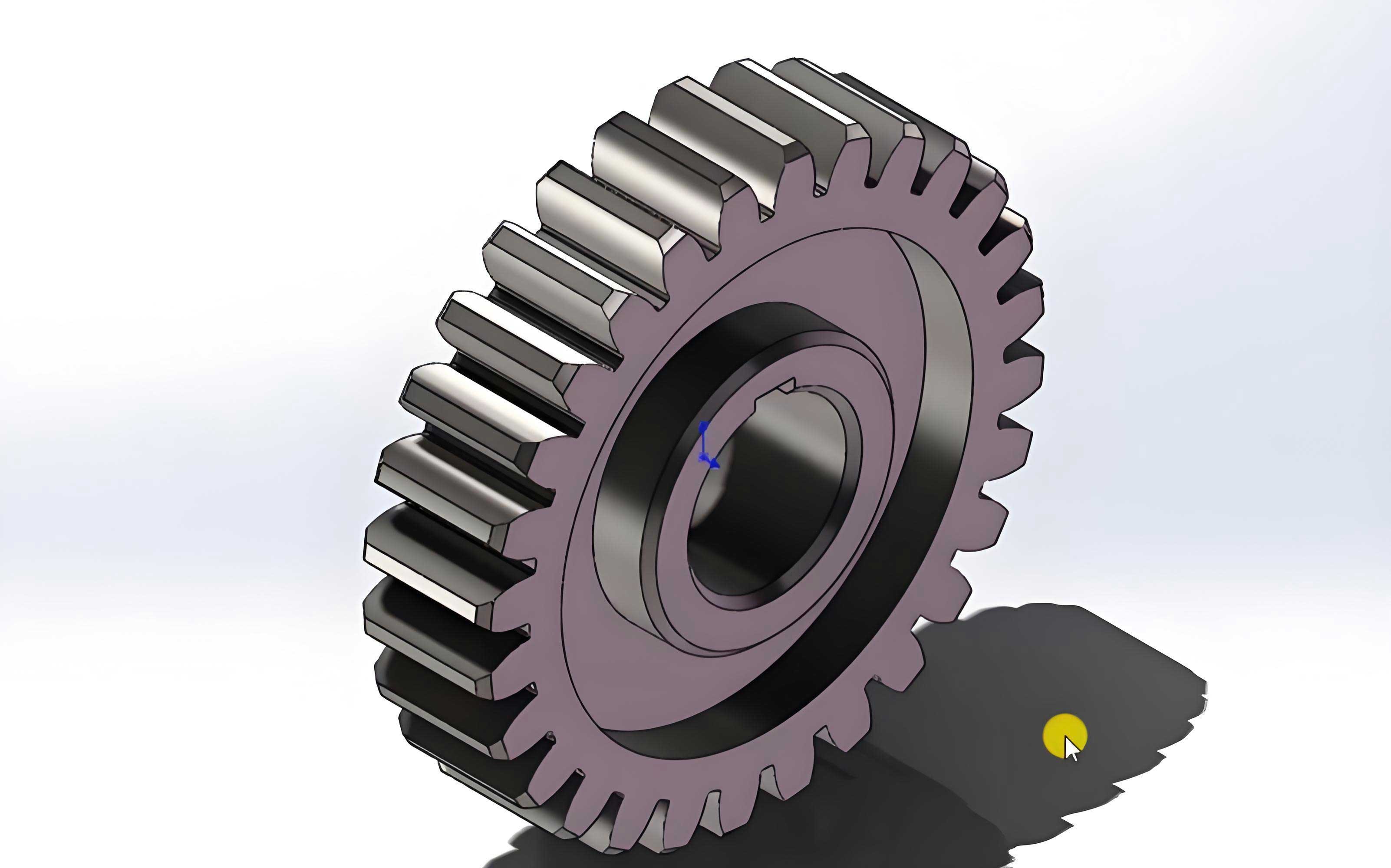
1. Introduction and Motivation
My research focuses on the nonlinear dynamic behavior of an internal meshing spur gear system (IMSGS), considering multi-state engagement and friction. As mechanical equipment advances toward intelligence and high power density, gear transmission systems face increasingly harsh service conditions. Internal spur gear drives, characterized by compact center distance, low contact stress, and high contact ratio, are widely used in planetary gear trains for wind turbines and other heavy-duty applications. However, the inherent nonlinear factors—such as time-varying backlash, time-varying mesh stiffness, and friction—induce complex vibration phenomena including tooth separation, back-side contact, bifurcation, and chaos.
Through my investigation, I have identified several critical research gaps in the existing literature. First, most dynamic models of spur gear systems simplify the backlash as a piecewise linear function or a simple harmonic function, ignoring the time-varying nature caused by elastic deformation, thermal deformation, and oil film thickness variation along the line of action (LoA). Second, prior studies on internal spur gears rarely classified the meshing states in detail, especially considering the coupling effect of contact ratio and time-varying backlash. Third, the global instability characteristics under parameter-initiation co-action have not been fully explored for internal spur gear pairs.
To address these issues, I developed a series of analytical models and conducted systematic numerical investigations. This paper presents my work on establishing a high-precision dynamic model of the IMSGS, exploring the multi-state meshing mechanism, and analyzing the global instability characteristics.
2. Dynamic Meshing Factor Modeling of Spur Gear System
2.1 Time-Varying Meshing Force Model
The accuracy of the contact force model significantly affects the dynamic response prediction of spur gear systems. Traditional linear spring-damper models, while widely used, fail to accurately capture the energy dissipation during meshing state transitions. Based on the Johnson contact force model, I proposed an improved dynamic meshing force calculation model for the internal spur gear system that incorporates energy dissipation. The meshing force can be expressed as:
$$F_m = \frac{(aD(\tau)+b)LE^*}{D(\tau)} x^n \left[1 + \frac{3(1-c_e^2)}{4} \cdot \frac{\dot{x}}{\dot{x}^{(-)}}\right]$$
(1)
where $D(\tau)$ is the time-varying backlash, $L$ is the center distance, $E^* = E/(2(1-\mu^2))$ is the comprehensive Young’s modulus, $x$ is the relative displacement along the LoA, $\dot{x}$ is the relative velocity, $\dot{x}^{(-)}$ is the initial relative velocity, and $c_e = 0.8$ is the restitution coefficient.
The parameters $a$, $b$, and $n$ depend on the magnitude of the backlash $\Delta R$ and can be summarized as shown in Table 2.1.
Table 2.1 Parameters of the improved contact force model for spur gear
| Parameter | $50\,\mu m < \Delta R \leq 10\,mm$ | $10\,mm < \Delta R < 500\,mm$ |
|:—:|:—:|:—:|
| $a$ | 0.965 | 0.39 |
| $b$ | 0.0965 | 0.85 |
| $n$ | $Y\Delta R^{-0.005}$ | 1.094 |
| $Y$ | $1.51[\ln(1000\Delta R)]^{-0.151}$ (for $0.005<\Delta R\leq0.34954$) | $0.151\Delta R+1.15$ (for $0.3954<\Delta R<10$) |
Thus, the meshing force can be rewritten in a compact form:
$$F_m = K_i x + c_i \dot{x}, \quad (i = k, d)$$
(2)
where the subscript $i=k$ denotes the drive-side (tooth face) meshing and $i=d$ denotes the back-side (tooth back) meshing. The equivalent stiffness $K_i$ and damping $c_i$ are:
$$K_i = \frac{(aD(\tau)+b)LE^*}{\Delta R}, \quad c_i = \frac{(aD(\tau)+b)LE^*}{D(\tau)} \cdot \frac{3(1-c_e^2)}{4\dot{x}^{(-)}}$$
(3)
2.2 Time-Varying Mesh Stiffness Model
The mesh stiffness model directly determines the accuracy of the spur gear dynamic model. I established a comprehensive time-varying mesh stiffness model that includes the elastic stiffness $k_e(t)$, the nonlinear Hertz contact stiffness $k_{eh}(t)$, and the thermal stiffness $k_t(t)$. The comprehensive mesh stiffness $k_m(t)$ is given by:
$$\frac{1}{k_m(t)} = \frac{1}{k_e(t)} + \frac{1}{k_{eh}(t)} + \frac{1}{k_t(t)}$$
(4)
The elastic stiffness $k_e(t)$ is composed of the bending stiffness $k_{eb}(t)$, shear stiffness $k_{es}(t)$, axial compressive stiffness $k_{ea}(t)$, and fillet-foundation stiffness $k_{ef}(t)$ for both the pinion and gear:
$$\frac{1}{k_e(t)} = \sum_{j=p,g} \left(\frac{1}{k_{ebj}(t)} + \frac{1}{k_{esj}(t)} + \frac{1}{k_{eaj}(t)} + \frac{1}{k_{efj}(t)}\right)$$
(5)
For the external spur gear (pinion), the stiffness components are calculated based on the potential energy method. The bending stiffness $k_{ebp}(t)$ and shear stiffness $k_{esp}(t)$ are expressed as:
$$\frac{1}{k_{ebp}(t)} = \int_{-\alpha_1}^{\alpha_3} \frac{3\{1+\cos\alpha_1[(\alpha_2-\alpha)\sin\alpha-\cos\alpha]\}^2(\alpha_2-\alpha)\cos\alpha}{2EB[\sin\alpha+(\alpha_2-\alpha)\cos\alpha]^3} d\alpha$$
(6)
$$\frac{1}{k_{esp}(t)} = \int_{-\alpha_1}^{\alpha_3} \frac{1.2(1+\mu)(\alpha_2-\alpha)\cos\alpha\cos^2\alpha_1}{EB[\sin\alpha+(\alpha_2-\alpha)\cos\alpha]^3} d\alpha$$
(7)
where $\mu$ is Poisson’s ratio, $B$ is the face width, and $E$ is Young’s modulus. The angles $\alpha_1$, $\alpha_2$, and $\alpha_3$ are determined by the gear geometry. Similarly, for the internal gear, the bending and shear stiffness are derived using a similar approach with the geometric parameters of the internal gear tooth.
The nonlinear Hertz contact stiffness, derived from the Hertz contact theory, is given by:
$$k_{eh}(t) = \frac{dF}{d\sigma} = 2E\sqrt{R\sigma}$$
(8)
where $R$ is the equivalent curvature radius and $\sigma$ is the contact deformation, defined as:
$$\sigma = \begin{cases} x – \bar{D}(\tau), & (x \geq \bar{D}(\tau)) \\ 0, & (|x| < \bar{D}(\tau)) \\ |x| – \bar{D}(\tau), & (x \leq -\bar{D}(\tau)) \end{cases}$$
(9)
The thermal stiffness, caused by tooth surface temperature rise, is expressed as:
$$k_{ti}(t) = F_n / \theta_{ti}(t), \quad (i = p, g)$$
(10)
where $\theta_{ti}(t)$ is the thermal deformation at the meshing point, which can be decomposed into radial thermal deformation $\theta_{tri}(t)$ and tooth thickness thermal deformation $\theta_{tsi}(t)$:
$$\theta_{ti}(t) = \theta_{tri}(t)\sin(\alpha_i(t)) + \theta_{tsi}(t)\cos(\alpha_i(t))$$
(11)
The radial and thickness thermal deformations are calculated by integrating the temperature field distribution. Figure 2.4 compares the elastic mesh stiffness with and without the nonlinear Hertz contact stiffness. My results show that incorporating the nonlinear Hertz contact stiffness makes the time-varying mesh stiffness smoother while slightly reducing its magnitude. The thermal stiffness $k_t(t)$ also contributes to reducing the comprehensive mesh stiffness, which is critical for accurate dynamic analysis of spur gear systems.
2.3 Time-Varying Damping Model
The meshing damping is closely related to the mesh stiffness. Based on the impact damping theory, I adopted the following time-varying damping model:
$$c_m(t) = \upsilon x^n = \frac{3(1-\psi)}{2\psi} \frac{k_m(t)}{\dot{x}^{(-)}} x^n$$
(12)
where $\upsilon$ is the hysteresis damping coefficient, $\psi = 0.7$ is the restitution coefficient, and $n = 1$ for the spur gear pair.
2.4 Multi-State Lubrication Friction Model
Friction between tooth surfaces significantly affects the dynamic behavior of spur gear systems. The lubrication state varies along the LoA depending on the oil film parameter $\Lambda(t)$:
$$\Lambda(t) = \frac{h(t)}{\sigma_r}$$
(13)
where $h(t)$ is the minimum oil film thickness and $\sigma_r$ is the composite surface roughness. Based on the value of $\Lambda(t)$, the lubrication state can be classified as:
- Elastohydrodynamic lubrication (EHL): $\Lambda(t) > 3.0$
- Mixed lubrication: $1.0 \leq \Lambda(t) \leq 3.0$
- Boundary lubrication: $\Lambda(t) < 1.0$
For each lubrication state, I established the corresponding friction coefficient model. Under EHL conditions, the friction coefficient is given by:
$$\mu_{Ei}(t) = \lambda_i(t) e^{f(SR_i(t),P_{hi}(t),\eta_M,R_{aavg})} P_{hi}^{b_2}(t) |SR_i(t)|^{b_3} (v_{ei}(t)/2)^{b_6} \eta_M^{b_7} \rho_{hi}^{b_8}(t)$$
(14)
where the function $f$ is:
$$f(SR_i(t), P_{hi}(t), \eta_M, R_{aavg}) = b_1 + b_9 e^{R_{aavg}} + b_4|SR_i(t)P_{hi}(t)\lg\eta_M| + b_5 e^{-|SR_i(t)P_{hi}(t)\lg\eta_M|}$$
(15)
The comprehensive multi-state lubrication friction model is expressed as:
$$\mu(t) = \begin{cases} \mu_E(t), & \Lambda(t) > 3.0 \\ \mu_M(t), & 1.0 \leq \Lambda(t) \leq 3.0 \\ \mu_C(t), & \Lambda(t) < 1.0 \end{cases}$$
(16)
where $\mu_M(t)$ is the mixed lubrication friction coefficient and $\mu_C(t) = 0.1$ is the constant boundary lubrication friction coefficient.
3. Nonlinear Dynamic Modeling of Internal Spur Gear System with Time-Varying Backlash and Multi-State Meshing
3.1 Classification of Meshing States
For an internal spur gear pair with a contact ratio $1 < \varepsilon_m < 2$, there exists periodic single-tooth and double-tooth alternation. Combined with the backlash-induced tooth separation and back-side contact, the gear system can exhibit five distinct meshing states. Based on the relative displacement $x$ along the LoA and the time-varying backlash $D(\tau)$, I classified the meshing states as follows:
Table 3.1 Classification of five meshing states and boundary conditions
| State | Description | Boundary Conditions |
|:—:|:—:|:—:|
| I | Double-tooth drive-side meshing | $x \geq D(\tau)$, $mT_0 \leq \tau \leq (\varepsilon-1)mT_0$ |
| II | Single-tooth drive-side meshing | $x \geq D(\tau)$, $(\varepsilon-1)mT_0 \leq \tau \leq (m+1)T_0$ |
| III | Double-tooth back-side meshing | $x \leq -D(\tau)$, $mT_0 \leq \tau \leq (\varepsilon-1)mT_0$ |
| IV | Single-tooth back-side meshing | $x \leq -D(\tau)$, $(\varepsilon-1)mT_0 \leq \tau \leq (m+1)T_0$ |
| V | Tooth separation (no contact) | $|x| < D(\tau)$, $mT_0 \leq \tau \leq (m+1)T_0$ |
3.2 Nonlinear Dynamic Model for Different Meshing States
Assuming rigid supports and considering only torsional vibration, I established the simplified physical model of the internal spur gear pair. Using Newton’s second law and the force analysis at the meshing points, I derived the relative torsional dynamics equations for each meshing state.
For the double-tooth drive-side meshing state:
$$m_e \ddot{\bar{x}} + [1 + \mu_{d1}(\tau)g_{d1}(\tau)L_{d1}(\tau) + \mu_{d2}(\tau)g_{d2}(\tau)L_{d2}(\tau)]F_m = \bar{F}_m + \bar{F}_h(\tau)$$
(17)
where $m_e = I_p I_g/(R_{bp}^2 I_p + R_{bg}^2 I_g)$ is the equivalent mass, $\bar{F}_m$ is the external load, $\bar{F}_h(\tau)$ is the internal error excitation, and $g_{di}(\tau)$ is the equivalent friction arm:
$$g_{di}(\tau) = \frac{R_{bp}I_p S_{dpi}(\tau) – R_{bg}I_g S_{dgi}(\tau)}{R_{bp}^2 I_p + R_{bg}^2 I_g}$$
(18)
For the single-tooth drive-side meshing state:
$$m_e \ddot{\bar{x}} + [1 + \mu_{d2}(\tau)g_{d2}(\tau)]F_m = \bar{F}_m + \bar{F}_h(\tau)$$
(19)
For the double-tooth back-side meshing state:
$$m_e \ddot{\bar{x}} – [1 + \mu_{b1}(\tau)g_{b1}(\tau)L_{b1}(\tau) + \mu_{b2}(\tau)g_{b2}(\tau)L_{b2}(\tau)]F_m = \bar{F}_m + \bar{F}_h(\tau)$$
(20)
For the single-tooth back-side meshing state:
$$m_e \ddot{\bar{x}} – [1 + \mu_{b2}(\tau)g_{b2}(\tau)L_{b2}(\tau)]F_m = \bar{F}_m + \bar{F}_h(\tau)$$
(21)
For the tooth separation state:
$$m_e \ddot{\bar{x}} = \bar{F}_m + \bar{F}_h(\tau)$$
(22)
3.3 Dimensionless Normalized Model
By introducing the meshing force function $f(\bar{x}, \bar{D}(\tau))$ and the meshing state function $h(\tau, \bar{x})$, I unified the five meshing state models into a single dimensionless normalized expression:
$$\ddot{x} + h(t, x)[k(t)f(x, D(t)) + c(t)\dot{x}] = F + \xi \omega^2 \cos(\omega t)$$
(23)
where $x = \bar{x}/D_c$, $\xi$ is the error coefficient, $\omega$ is the dimensionless meshing frequency, and $F$ is the dimensionless load. The meshing state function $h(t, x)$ is defined piecewise according to the five meshing states, and the parameters used in my simulations are summarized in Table 3.2.
Table 3.2 Parameters of the internal spur gear system
| Parameter | Symbol | Value |
|:—:|:—:|:—:|
| Teeth number (pinion/gear) | $z_p/z_g$ | 30/70 |
| Module | $m$ | 3 mm |
| Pressure angle | $\alpha$ | 20° |
| Face width | $B$ | 25 mm |
| Young’s modulus | $E$ | 210 GPa |
| Poisson’s ratio | $\mu$ | 0.30 |
| Average mesh stiffness | $k_{av}$ | $4\times10^8$ N/m |
| Damping ratio | $\xi$ | 0.07 |
| Characteristic size | $D_c$ | 100 μm |
4. Multi-State Meshing Mechanism and Nonlinear Dynamic Characteristics
4.1 Phase Plane Partition and Poincaré Maps
Based on the time-varying backlash, I divided the phase plane into five distinct regions, as illustrated in Figure 4.1. In the phase plane, $D_d$ and $D_s$ denote the half-values of the backlash in the double-tooth and single-tooth meshing regions, respectively, with $D_s > D_d$.
To effectively characterize the multi-state meshing behavior, I defined five types of Poincaré sections:
- Time periodic section: $\Omega_n = \{(x, \dot{x}, t) \in \mathbb{R}^2 \times \mathbb{R}_+, \text{mod}(t, 2\pi/\omega) = 0\}$
- Single-tooth drive-side impact section: $\Omega_p = \{(x, \dot{x}, t) \in \mathbb{R}^2 \times \mathbb{R}_+, x = D_s\}$
- Single-tooth back-side impact section: $\Omega_q = \{(x, \dot{x}, t) \in \mathbb{R}^2 \times \mathbb{R}_+, x = -D_s\}$
- Double-tooth drive-side impact section: $\Omega_r = \{(x, \dot{x}, t) \in \mathbb{R}^2 \times \mathbb{R}_+, x = D_d\}$
- Double-tooth back-side impact section: $\Omega_s = \{(x, \dot{x}, t) \in \mathbb{R}^2 \times \mathbb{R}_+, x = -D_d\}$
The system’s multi-state meshing behavior can be characterized by the symbol $n-p-q-r-s$, where $n$ is the number of motion periods, $p$ is the number of single-tooth drive-side impacts, $q$ is the number of single-tooth back-side impacts, $r$ is the number of double-tooth drive-side impacts, and $s$ is the number of double-tooth back-side impacts over one period.
4.2 Multi-State Meshing Mechanism
To reveal the generation mechanism of tooth separation and back-side meshing, I examined the dynamic meshing force and relative displacement along the LoA. Figure 4.3 illustrates the transition process from drive-side meshing to tooth separation.
The mechanism can be described as follows: The dynamic meshing force in the single-tooth region first decreases to zero, then reverses direction (becomes negative), indicating a tendency for the meshing tooth pair to separate. However, as long as the relative displacement remains larger than the half-backlash in the single-tooth region ($x > D_s$), the tooth pair remains in contact. Only when the relative displacement equals $D_s$ does the single-tooth drive-side meshing force abruptly drop to zero, and the system transitions to tooth separation in the single-tooth region. Subsequently, the double-tooth meshing force also decreases to zero and reverses direction, until the relative displacement equals $D_d$. At this point, the double-tooth meshing force also drops to zero, and the system completely transitions to the tooth separation state.
4.3 Influence of Backlash D on Multi-State Meshing Behavior
Using the dimensionless system parameters $\xi = 0.27$ and $\omega = 1.4$, I investigated the evolution of multi-state meshing behavior as a function of the static backlash $D$. The bifurcation diagrams on different Poincaré sections and the corresponding TLE spectrum are shown in Figure 4.4.
When the backlash is small, the spur gear system exhibits stable 1-1-1-1-1 motion, with the phase trajectory crossing $D_s$, $D_d$, $-D_s$, and $-D_d$. The dynamic meshing force alternates periodically between positive (drive-side meshing), zero (tooth separation), and negative (back-side meshing) values.
As the backlash increases, the 1-1-1-1-1 motion undergoes a bifurcation at point A to 2-1-1-1-1 motion. At point B, a period-doubling bifurcation leads to 4-2-2-2-2 motion. The period-4 motion then transitions to period-2 motion at point C via a reverse period-doubling bifurcation. At point D, the stable 2-1-1-1-1 behavior enters chaos, with the corresponding TLE becoming positive. At point E, the chaotic motion degenerates to period-3 motion, which then re-enters chaos at point F.
These results indicate that the static backlash significantly affects the multi-state meshing characteristics of the spur gear system. For large backlashes, the system exhibits coexisting periodic and chaotic motions with stronger nonlinear characteristics. Therefore, the static backlash should be minimized while ensuring proper lubrication and preventing tooth seizure.
4.4 Influence of Transmission Error Coefficient ξ
The transmission error coefficient $\xi$ also plays a critical role in the multi-state meshing behavior of internal spur gears. With $F = 0.05$ and $\omega = 1.5$, I calculated the bifurcation diagrams on different Poincaré sections and the corresponding TLE spectrum as shown in Figure 4.6.
When $\xi$ is small, the spur gear system exhibits constant 1-0-0-1-0 motion with stable mesh behavior. As $\xi$ increases, an incomplete bifurcation occurs at point A, leading to the coexistence of 1-0-0-1-0 and 2-1-0-1-0 behaviors. The period-1 motion persists with relatively small relative displacement, slightly crossing the boundary $D_d$, while the period-2 motion exhibits more pronounced dynamic meshing force variations.
At point B, another incomplete bifurcation occurs, producing a new period-2 motion and 3-1-0-1-0 behavior, while the original 2-1-0-1-0 behavior continues without bifurcation. Consequently, two period-2 motions and a period-3 motion coexist. At point C, a complete bifurcation leads to 4-2-0-2-0 behavior.
In the range of $\xi \in (0.044, 0.126)$, the spur gear system exhibits complex dynamic behaviors including chaos, period-doubling bifurcations, and multi-state meshing. The appearance of back-side meshing and tooth separation states is closely related to the bifurcation transitions. The five-state meshing behavior is frequently observed when the response becomes chaotic or exhibits large-amplitude periodic oscillations.
4.5 Maximum Dynamic Meshing Force in the Dual-Parameter Plane
To understand the coupled influence of transmission error and load on the meshing behavior, I calculated the maximum dynamic meshing force in the $(\xi, F)$ parameter plane, as shown in Figure 4.8(a). The results reveal that:
- When both $\xi$ and $F$ are small, the maximum dynamic meshing force shows slight fluctuations, indicating relatively stable meshing behavior.
- When $\xi > 0.2$ and $F > 0.175$, the maximum dynamic meshing force gradually reaches its peak value $F_{max} = 1.340$.
- Significant fluctuations of the maximum meshing force are observed in $\xi \in (0.044, 0.126)$, $\xi \in (0.236, 0.3)$, $F \in (0, 0.007)$, and $F \in (0.055, 0.095)$, which coincide with the regions where the spur gear system exhibits chaotic and back-side meshing behaviors.
Table 4.1 Summary of multi-state meshing behavior vs. parameters for the spur gear pair
| Parameter Range | System Behavior | Meshing States |
|:—:|:—:|:—:|
| Small $D$ or small $\xi$ | 1-1-1-1-1 or 1-0-0-1-0 | Drive-side meshing + separation |
| Medium $D$ or medium $\xi$ | 2-1-1-1-1, 4-2-2-2-2 | Multi-state with back-side meshing |
| Large $D$ or large $\xi$ | Chaos, 3-1-1-1-1 | Five-state meshing, complex switching |
5. Global Instability Characteristics of Internal Spur Gear System
5.1 Identification of Multi-State Meshing Behavior
To effectively identify the multi-state meshing behavior, I defined the Poincaré sections $\Pi_s$ and $\Pi_b$ as:
$$\Pi_s = \{(x,t) | (x,t) \in \mathbb{R}^3 \times \mathbb{R}, x_1 = D\}$$
(24)
$$\Pi_b = \{(x,t) | (x,t) \in \mathbb{R}^3 \times \mathbb{R}, x_2 = -D\}$$
(25)
If $\Pi_s \cap \Gamma = \emptyset$ and $\Pi_b \cap \Gamma = \emptyset$, where $\Gamma$ denotes the phase trajectory, the spur gear system exhibits only drive-side meshing without tooth separation or back-side contact. Otherwise, the system may experience tooth separation or back-side meshing states.
5.2 Time-Domain Calculation Method for Dynamic Instability Cycle Ratio
I proposed a time-domain calculation method to quantify the dynamic instability of the spur gear system. The phase plane $x-\dot{x}$ is divided into three regions: the drive-side meshing region ($x > D$), the tooth separation region ($|x| < D$), and the back-side meshing region ($x < -D$). The dynamic instability cycle ratio $P_{ID}$ can be calculated as:
$$P_{ID} = \frac{t_s + t_b}{t_d + t_s + t_b}$$
(26)
where $t_d$ is the duration of drive-side meshing, $t_s$ is the duration of tooth separation, and $t_b$ is the duration of back-side meshing. These durations are computed as:
$$t_d = \sum_{n} h N_d^n (x_n > D), \quad t_s = \sum_{n} h N_s^n (|x_n| < D), \quad t_b = \sum_{n} h N_b^n (x_n < -D)$$
(27)
where $h$ is the time step of the Runge-Kutta method, and $N_d$, $N_s$, $N_b$ are the iteration counts in each region.
5.3 Global Instability under the Influence of Meshing Frequency ω
With system parameters $F = 0.07$ and $\xi = 0.23$, I calculated the multi-initial bifurcation diagrams and the corresponding TLE spectra as functions of $\omega$, as shown in Figure 5.3. The evolution of coexisting attractors is summarized in Table 5.1.
Table 5.1 Evolution of attractors with increasing mesh frequency ω for internal spur gear pair
| $\omega$ range | Figure | Healthy attractors | Unstable attractors |
|:—:|:—:|:—:|:—:|
| $\omega \in (0.01, 0.42)$ | — | P1 (H) | — |
| $\omega \in (0.421, 0.54)$ | 5.5(b) | P1 (H) | Q1 (In) |
| $\omega \in (0.541, 0.58)$ | — | R1 (H) | Q1 (In) |
| $\omega \in (0.581, 0.63)$ | 5.5(d) | R2 (In) | Q1 (In) |
| $\omega \in (0.631, 0.72)$ | — | Q1 (In) | — |
| $\omega \in (0.72, 1.26)$ | — | QN (In) | — |
| $\omega \in (1.261, 1.526)$ | — | Q2 (H) | PN (In) |
| $\omega \in (1.802, 1.891)$ | 5.5(f) | Q2 (H) | P3 (In) |
| $\omega \in (1.891, 2.304)$ | 5.5(h) | Q1 (H) | P3 (In) |
| $\omega \in (2.304, 3.0)$ | — | Q1 (H) | — |
When $\omega$ is small (left of point A), the spur gear system exhibits stable 1-0-0-1-0 behavior with single-tooth separation and double-tooth drive-side meshing. At $\omega = 0.364$, an incomplete bifurcation occurs at G1, resulting in the coexistence of 1-0-0-1-0 behavior (P1) and 1-1-1-1-1 behavior (Q1). The attraction basin shown in Figure 5.5(b) reveals that the healthy period P1 accounts for 49% of the basin area, while the unstable period Q1 accounts for 51%.
As $\omega$ increases, P1 undergoes another incomplete bifurcation at point G2, producing a new period-1 motion R1. At point A, R1 undergoes a period-doubling bifurcation to R2, while Q1 continues without bifurcation. At point B, R2 transitions into chaos while Q1 persists, resulting in coexisting Q1 and chaotic responses. At point C, the chaotic response degenerates to Q1, and only Q1 exists. When $0.72 < \omega < 1.5$, the system enters various chaotic states with frequent occurrences of multi-state meshing behavior.
In the range $\omega \in (1.261, 1.526)$, the system exhibits stable 3-1-1-1-1 behavior (P3) coexisting with unstable chaotic motion (PN). At $\omega = 1.801$ (point G3), the coexistence of P3 and 2-1-0-2-0 behavior (Q2) is observed. The unstable period P3 accounts for 84% of the basin area, while the stable period Q2 accounts for 16%. At point F ($\omega = 1.812$), Q2 transitions to Q1 through an inverse period-doubling bifurcation, resulting in the coexistence of P3 and Q1.
The spur gear system’s attractors are highly sensitive to initial values in certain parameter ranges. For instance, when $P_3$ exists, slight perturbations in initial values can cause continuous switching between P3 and Q1, significantly affecting the global dynamic characteristics.
5.4 Global Instability under the Influence of Load F
Taking system parameters $\omega = 1.4$ and $\xi = 0.09$, I calculated the multi-initial bifurcation diagrams and TLE spectra as functions of the load $F$, as shown in Figure 5.6. The evolution of coexisting attractors is summarized in Table 5.2.
Table 5.2 Evolution of attractors with increasing load F for internal spur gear pair
| $F$ range | Figure | Healthy attractors | Unstable attractors |
|:—:|:—:|:—:|:—:|
| $F \in (0.0001, 0.0021)$ | 5.8(b) | — | P3 (In), PN (In) |
| $F \in (0.0022, 0.035)$ | — | — | P3 (In) |
| $F \in (0.036, 0.042)$ | — | — | P6 (In) |
| $F \in (0.043, 0.045)$ | — | — | P10 (In) |
| $F \in (0.046, 0.089)$ | — | — | PN (In) |
| $F \in (0.09, 0.104)$ | 5.8(c) | P2 (H), Q4 (H) | P3 (In) |
| $F \in (0.105, 0.117)$ | 5.8(e) | P2 (H), Q2 (H) | P3 (In) |
| $F \in (0.118, 0.2)$ | 5.8(g) | P1 (H), Q2 (H) | — |
When $F$ is large (right of point G3), the spur gear system exhibits stable 1-1-0-1-0 behavior (P1) coexisting with 2-1-0-1-0 behavior (Q2). The healthy period P1 accounts for 78% of the basin area, while the stable period Q2 accounts for 22%.
At $F = 0.117$ (point G3), P1 undergoes an incomplete bifurcation, producing R3 and P2. Between G3 and G2, the system exhibits the coexistence of P3 (17%), Q2 (62%), and P2 (21%), as shown in Figure 5.8(d). The attractor basins exhibit a sieve-like distribution, indicating complex global dynamics.
At point G2 ($F = 0.1044$), Q2 undergoes a period-doubling bifurcation to Q4, while P3 and P2 continue without bifurcation. The unstable period R3 grows to 58% of the basin area. When $F$ decreases to point G1, P3, Q2, and P4 transition to chaos through a series of period-doubling bifurcations.
For the chaotic spur gear system, the dynamic meshing force can be greater than or equal to zero without the presence of negative values, proving that chaos is not entirely caused by back-side meshing behavior. The chaotic attractor expands significantly when back-side meshing and tooth separation occur. The system later degenerates from chaos to 12-4-4-4-4 behavior through a saddle-node bifurcation at point E, then transitions to 6-2-2-2-2 behavior through a reverse period-doubling bifurcation at point D, and finally to 3-1-1-1-1 behavior at point B.
5.5 Bifurcation and Safety Tree Diagram
Figure 5.5 and Figure 5.8 illustrate the bifurcation and safety tree diagrams for the internal spur gear system as functions of $\omega$ and $F$, respectively. These diagrams summarize the complete bifurcation scenarios, incomplete bifurcations, and parameter ranges where coexisting attractors exist.
The key findings from my analysis are:
- Incomplete bifurcations are the primary mechanism generating coexisting attractors in the internal spur gear system. These bifurcations are governed by the synergistic action of parameters and initial state space.
- The multi-state meshing behavior evolution is intrinsically linked to the bifurcation structure. Tooth separation and back-side meshing states emerge when the system undergoes incomplete or complete bifurcations.
- Coexisting periodic motions exhibit different sensitivities to initial conditions. Some attractors are extremely sensitive, where small perturbations can induce switching between different meshing states, leading to unpredictable dynamic behavior.
6. Conclusion
In this paper, I investigated the nonlinear dynamic behavior of an internal meshing spur gear system considering multi-state engagement and friction. The following conclusions are drawn:
(1) I established comprehensive dynamic meshing factor models for the internal spur gear system, including an improved Johnson-based contact force model with energy dissipation, a time-varying mesh stiffness model incorporating nonlinear Hertz contact stiffness and thermal stiffness, and a multi-state lubrication friction model covering EHL, mixed, and boundary lubrication regimes. The results demonstrate that both the nonlinear Hertz contact stiffness and thermal deformation stiffness reduce the comprehensive time-varying mesh stiffness. The elastic stiffness and comprehensive stiffness both increase then decrease along the line of action, with jumps at the single-tooth and double-tooth alternation points. Considering the strong nonlinearity of the system, the time-varying backlash jumps during single/double-tooth alternation, with larger half-backlash in the single-tooth region compared to the double-tooth region.
(2) Based on the coupling effects of time-varying backlash and contact ratio, I classified the meshing states of the spur gear system into five types: single-tooth drive-side, double-tooth drive-side, single-tooth back-side, double-tooth back-side, and tooth separation. A dimensionless normalized nonlinear dynamic model was established for the internal spur gear system considering time-varying backlash and multi-state meshing. The dynamic meshing force mutation in the direction is the main cause of tooth separation and back-side meshing. Tooth separation can occur in either the single-tooth or double-tooth meshing region, with the dynamic meshing force undergoing one or two mutations, respectively.
(3) The system parameters (backlash, transmission error, meshing frequency, and load) significantly affect the multi-state meshing characteristics and nonlinear dynamic behavior of the internal spur gear system. The maximum dynamic meshing force exhibits significant fluctuations in the dual-parameter ($\xi$-$F$) plane when the spur gear system exhibits complex bifurcation or chaotic states, such as $\xi \in (0.044, 0.126)$ and $F \in (0.055, 0.095)$. The peak value of the maximum dynamic meshing force occurs when both $\xi$ and $F$ are large.
(4) Incomplete bifurcation, governed by parameter-state space synergistic actions, is the primary reason for behavior coexistence, increasing the number of coexisting attractors in the internal spur gear system. Some periodic motions show strong sensitivity to initial values, where slight perturbations can cause switching between meshing states. When multiple solutions coexist, selecting a specific periodic motion’s initial value can prevent other periodic motions from appearing, thereby improving the safety and stability of the spur gear system. These findings provide theoretical guidance for predicting and controlling the dynamic behaviors of spur gear transmission systems, improving dynamic performance, and optimizing parameter design.