
1. Introduction and Research Background
In recent years, the rapid development of the automotive industry has led to a continuously increasing demand for gears. Traditional cutting processes suffer from low material utilization and poor production efficiency, which contradicts the principles of sustainable development. Precision forging forming technology, in contrast, offers high material utilization, high production efficiency, and superior product quality. Therefore, it is imperative that precision forging replaces conventional machining. In my research, I employed three-dimensional elastic-plastic finite element simulation methods to model the cold precision forging process of a straight bevel gear, obtaining deformation data for both the die and the forging.
The cold precision forging of a straight bevel gear involves extremely high forming resistance. During the forming process, the die undergoes elastic deformation, and the forging experiences elastic springback after ejection from the die. These two elastic deformation behaviors significantly influence the accuracy of the cold-forged gear. My work focuses on improving the precision of cold-forged straight bevel gears by applying a reverse compensation method to modify the die cavity, thereby eliminating these adverse effects and ultimately obtaining a straight bevel gear forging that meets required precision standards. The primary tasks are summarized below.
2. Elastic-Plastic Finite Element Theory
2.1 Fundamental Concepts
Metal volume forming is characterized by large displacements and large strains. When analyzing the forming process with finite element methods, the material model selection is critical. The elastic-plastic finite element method (FEM) reflects the true constitutive behavior of metallic materials during large deformation more accurately than rigid-plastic or rigid-viscoplastic models. This is particularly important for predicting residual stresses and springback. The method is based on the incremental theory of plasticity, which includes the yield criterion, flow rule, and hardening law.
2.2 Yield Criterion
For elastic-plastic analysis, the von Mises yield criterion is commonly adopted. It states that yielding begins when the equivalent stress reaches the yield strength of the material:
$$ \bar{\sigma} = \frac{1}{\sqrt{2}} \sqrt{(\sigma_x – \sigma_y)^2 + (\sigma_y – \sigma_z)^2 + (\sigma_z – \sigma_x)^2 + 6(\tau_{xy}^2 + \tau_{yz}^2 + \tau_{zx}^2)} = \sigma_s \tag{2-1} $$
2.3 Plastic Flow Rule and Hardening Law
The Prandtl-Reuss flow rule is used to describe the elastic-plastic constitutive relationship. The total strain increment is decomposed into elastic and plastic components:
$$ \{d\varepsilon\} = \{d\varepsilon^e\} + \{d\varepsilon^p\} \tag{2-2} $$
For hardening materials, the subsequent yield surface depends on the total equivalent plastic strain. The incremental stress-strain relationship in matrix form is given by:
$$ \{d\sigma\} = [D^{ep}] \{d\varepsilon\} \tag{2-3} $$
where $[D^{ep}]$ is the elastic-plastic matrix, which is a function of the stress state and deformation history.
2.4 Finite Element Equations
For large deformation problems, the principle of virtual work in incremental form is employed:
$$ \int_V [\delta\varepsilon]^T [D^{ep}] \{\Delta\varepsilon\} \, dV = \int_V \{\delta u\}^T \{\Delta b\} \, dV + \int_S \{\delta u\}^T \{\Delta p\} \, dS – \int_V \{\delta\varepsilon\}^T \{\sigma\} \, dV \tag{2-4} $$
The global finite element equation is then expressed as:
$$ [K^{ep}] \{\Delta\delta\} = \{\Delta F\} \tag{2-5} $$
where $[K^{ep}]$ is the elastic-plastic stiffness matrix, $\{\Delta\delta\}$ is the nodal displacement increment vector, and $\{\Delta F\}$ is the external force increment vector.
3. Three-Dimensional Modeling of the Straight Bevel Gear
3.1 Gear Geometric Parameters
The research object is a planetary gear and a side gear used in an automotive differential. The key geometric parameters of the planetary gear are presented in Table 1 and Table 2.
Table 1: Planetary gear tooth parameters
| Parameter | Value |
|---|---|
| Module | 5 mm |
| Number of teeth | 10 |
| Pressure angle | 22°30′ |
| Shaft angle | 90° |
| Full tooth height | 8.94 mm |
| Pitch diameter | 65 mm |
| Tip cone angle | 45°28′ |
| Pitch cone angle | 37°34′ |
| Root cone angle | 31°44′ |
| Effective tooth height | 8 mm |
Table 2: Side gear tooth parameters
| Parameter | Value |
|---|---|
| Module | 5 mm |
| Number of teeth | 10 |
| Pressure angle | 22°30′ |
| Shaft angle | 90° |
| Full tooth height | 8.94 mm |
| Pitch diameter | 65 mm |
| Tip cone angle | 58°16′ |
| Pitch cone angle | 52°26′ |
| Root cone angle | 44°32′ |
| Effective tooth height | 8 mm |
3.2 Forging Design
When designing the forging for the straight bevel gear, I established the parting surface at the intersection of the back cone surface and the gear bottom to prevent the die from collapsing the tooth tips. Machining allowances of 0.5 mm were reserved on the back cone and free forging surfaces. The fillet radii were calculated using empirical formulas commonly applied in closed precision forging. For the planetary gear, the upper punch draft angle is 30°, the lower punch is 10°, and the side gear uses 30° for the upper punch and 15° for the lower punch.
3.3 Parametric Modeling Using B-Spline Surfaces
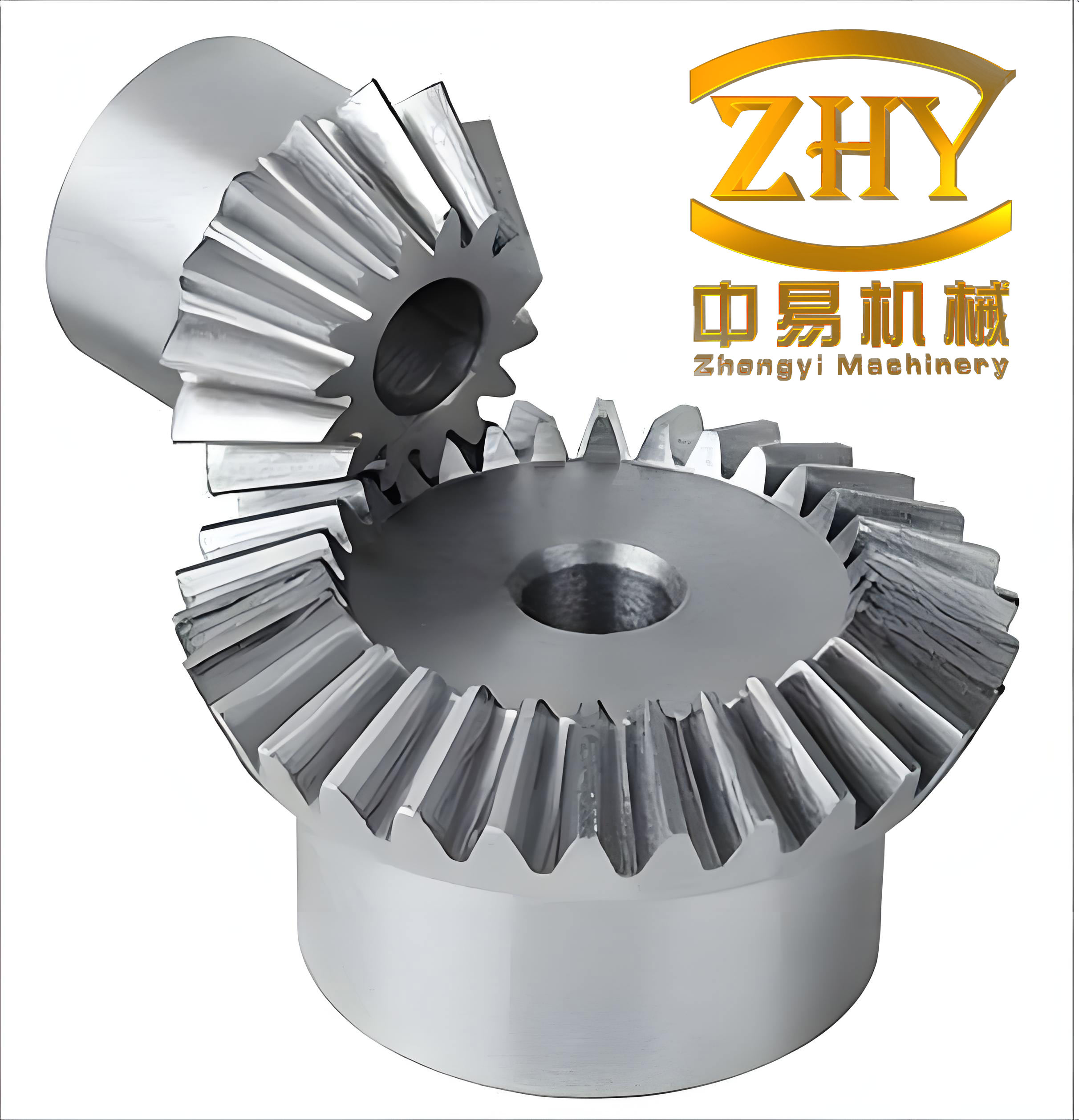
To model the straight bevel gear accurately, I constructed a grid of $m \times n$ points on the tooth flank and generated the tooth surface using the B-spline method. The complete three-dimensional model was then created in the UG software environment. This approach closely simulates the machining process and ensures high precision of the tooth profile. The forging model of the straight bevel gear and the corresponding die cavity model were both established with parametric design capability for subsequent modifications.
4. Optimization of the Cold Forging Process
4.1 Preform Design
Considering the forming characteristics of the straight bevel gear, the process can be divided into upsetting and extrusion. The planetary gear, having fewer teeth and a smaller diameter, can be forged directly in one step. The side gear, with more complex geometry and higher forming resistance, requires a preforming step. Based on the constant volume principle, I designed a cylindrical preform with a tapered top for the side gear, as shown in Table 3.
Table 3: Preform dimensions for the side gear
| Parameter | Value (mm) |
|---|---|
| Maximum diameter | 35 |
| Bottom diameter | 28 |
| Top diameter | 16 |
| Total height | 26 |
4.2 Lubrication
Lubrication plays a critical role in the cold precision forging of straight bevel gears. The contact pressure between the die and the workpiece can reach 800–1100 MPa, sometimes up to 2400 MPa. Conventional phosphate-soap coating may crack due to the significant surface area changes during forging. I adopted a combination of phosphate coating and a water-based graphite lubricant, achieving a friction coefficient of approximately 0.12, which is reasonable for industrial production.
4.3 Die Structure Design
The die structure for cold precision forging of a straight bevel gear must withstand enormous forces. Based on the allowable unit pressure, I selected a two-layer combined die structure with an interference of 0.45 mm and an axial pressing amount of 10 mm, as presented in Table 4.
Table 4: Combined die design parameters
| Parameter | Value |
|---|---|
| Interference | 0.45 mm |
| Axial pressing amount | 10 mm |
| Die material (inner) | High-strength alloy steel |
| Prestress ring material | SKD11 |
| Total diameter ratio | 4–6 |
The complete die assembly consists of the tooth-shaped die, upper punch, lower punch, and back cone die. The upper and lower punches are made of high-strength alloy steel, and thick backing plates are placed at both ends to enhance overall rigidity. The three-dimensional models of the die components are shown in Figure 3.
4.4 Finite Element Model Setup
Considering the cyclic symmetry of the straight bevel gear, I modeled only one-tenth of the gear to reduce computational time while preserving accuracy. The finite element model was established in DEFORM-3D. The key simulation parameters are listed in Table 5.
Table 5: Simulation parameters for cold precision forging of straight bevel gear
| Parameter | Value |
|---|---|
| Workpiece material | 20CrMnTi (substituted by 20MnCr5) |
| Die material | Elastic body |
| Punch velocity | 30 mm/s |
| Friction coefficient | 0.12 |
| Initial temperature | 20 °C |
| Environment temperature | 20 °C |
| Number of elements | 50,000 |
| Minimum element size | 0.3 mm |
| Time step length | 0.1 mm |
4.5 Comparison of Forging Process Schemes
To optimize the forming process for the straight bevel gear, I compared three different schemes: (1) closed die forging, (2) open die forging with flash gutter, and (3) a combined open-closed die forging process. The load-stroke curves for the three schemes were compared, and the results are summarized in Table 6.
Table 6: Comparison of forging process schemes
| Scheme | Maximum load (×10⁵ N) | Filling quality | Springback level |
|---|---|---|---|
| Closed die forging | 5.94 | Excellent | High |
| Open die forging | 4.46 | Poor | Low |
| Combined open-closed | 5.46 | Excellent | Medium |
The combined process, which starts as an open die forging and transitions to closed die forging after the die cavity closes, significantly reduces the forming load by approximately 10% compared to fully closed die forging, while maintaining comparable forging quality. This new process effectively balances formability and dimensional accuracy for the straight bevel gear. Additionally, I observed that the springback of the gear forging is proportional to the forming load, with the relationship becoming more pronounced at higher loads.
5. Elastic Deformation and Springback Analysis
5.1 Simulation Strategy
Traditional approaches often treat the die as a rigid body during forming and then separately analyze the die deformation based on the contact stress distribution. However, this method neglects the interaction between die deformation and workpiece springback. In my research, I treated the die as an elastic body from the beginning of the simulation, and the workpiece as an elastic-plastic body. This coupled approach more accurately reflects the actual forging conditions.
5.2 Die Cavity Elastic Deformation
To analyze the elastic deformation of the die cavity, I extracted 9 tooth profile curves from the small end to the large end of the tooth cavity, with 5 nodes equally distributed on each curve. By tracking the displacement of these nodes during the forming process, I obtained the deformation pattern of the die cavity. The key findings are as follows:
- On each tooth profile curve of the die cavity, the deformation is largest at the tooth tip and decreases toward the tooth root, reaching a minimum at the widest part (the drum-shaped area), then increases slightly toward the root.
- Across the entire die cavity, the elastic deformation is largest at the small end of the straight bevel gear and gradually decreases toward the large end.
Table 7 presents the elastic deformation values at selected nodes on the first and ninth tooth profile curves for the straight bevel gear die cavity.
Table 7: Die cavity elastic deformation distribution (mm)
| Node position | Curve 1 (small end) | Curve 9 (large end) |
|---|---|---|
| Tooth tip | 0.152 | 0.098 |
| Near tip | 0.134 | 0.087 |
| Middle | 0.118 | 0.079 |
| Near root | 0.124 | 0.084 |
| Tooth root | 0.141 | 0.092 |
5.3 Gear Forging Springback
The elastic springback of the straight bevel gear forging was studied using a similar methodology. After the forming simulation, I analyzed the nodal displacements when the die was removed. The springback pattern of the gear forging is consistent with the die deformation pattern, which confirms the strong correlation between them. The maximum springback occurs at the tooth tip of the small end, with a value of approximately 0.149 mm. The springback at the drum-shaped area is close to zero, and it gradually increases toward both the tooth tip and the tooth root.
Table 8: Springback values at different tooth profile positions (mm)
| Position | Small end | Middle | Large end |
|---|---|---|---|
| Tooth tip | 0.149 | 0.118 | 0.086 |
| Working profile (upper) | 0.121 | 0.095 | 0.069 |
| Drum-shaped area | 0.018 | 0.012 | 0.007 |
| Working profile (lower) | 0.055 | 0.041 | 0.030 |
| Tooth root | 0.087 | 0.066 | 0.048 |
5.4 Data Processing Method
To accurately extract the nodal displacement data from the simulation results, I imported the deformed mesh data into HyperMesh software. By intersecting planes with the gear model at the positions of the 9 tooth profile curves, I obtained intersection lines on the working tooth surface. The nodal coordinates on these lines were then exported and compared with the theoretical model coordinates using MATLAB. This approach avoided the issue of node renumbering caused by mesh remeshing and provided reliable deviation values for each point on the tooth surface.
6. Tooth Surface Accuracy Inspection and Die Cavity Modification
6.1 Accuracy Inspection Method
For the straight bevel gear, dimensional accuracy alone is insufficient to guarantee proper performance. The tooth surface contact pattern is equally important for transmission efficiency and gear life. After each iteration of die modification, I performed both dimensional accuracy inspection and tooth contact analysis on the simulated forging. The contact analysis was based on the gear meshing theory, ensuring that the modified tooth surface meets the conjugate contact conditions.
6.2 Reverse Compensation Modification Method
I adopted the single-amplitude reverse compensation iterative method to modify the die cavity. The procedure is as follows:
- Extract the deviation values of the 5×9 control points that define the B-spline surface of the tooth flank.
- Compensate each point by an amount equal to its deviation value in the opposite direction.
- Fit the compensated discrete points to obtain new tooth profile curve equations.
- Generate the new tooth surface and apply smoothing twice to eliminate surface irregularities.
- Construct the modified die cavity model and perform the finite element simulation again.
- Inspect the accuracy of the new forging. If it meets the precision requirement, stop; otherwise, repeat the process.
The deviation values of the B-spline surface control points after each modification step are summarized in Table 9–11. Initially, the maximum deviation was 0.1493 mm. After the first modification, the maximum deviation decreased to 0.1046 mm (in the negative direction). After the second modification, the deviation values were all within ±0.030 mm, which satisfies the national standard grade 7 precision for the straight bevel gear.
Table 9: Initial deviation values of B-spline control points (mm)
| Curve | Node 1 | Node 2 | Node 3 | Node 4 | Node 5 |
|---|---|---|---|---|---|
| 1 | 0.1209 | 0.0995 | 0.0773 | 0.0541 | 0.0297 |
| 2 | 0.1344 | 0.1049 | 0.0774 | 0.0516 | 0.0273 |
| 3 | 0.1436 | 0.1083 | 0.0770 | 0.0492 | 0.0250 |
| 4 | 0.1486 | 0.1099 | 0.0762 | 0.0471 | 0.0226 |
| 5 | 0.1493 | 0.1095 | 0.0749 | 0.0453 | 0.0202 |
| 6 | 0.1457 | 0.1072 | 0.0733 | 0.0436 | 0.0179 |
| 7 | 0.1378 | 0.1030 | 0.0713 | 0.0422 | 0.0156 |
| 8 | 0.1256 | 0.0970 | 0.0688 | 0.0410 | 0.0133 |
| 9 | 0.1092 | 0.0890 | 0.0660 | 0.0401 | 0.0110 |
Table 10: Deviation values after first modification (mm)
| Curve | Node 1 | Node 2 | Node 3 | Node 4 | Node 5 |
|---|---|---|---|---|---|
| 1 | -0.0606 | -0.0552 | -0.0473 | -0.0371 | -0.0242 |
| 2 | -0.0741 | -0.0634 | -0.0511 | -0.0371 | -0.0212 |
| 3 | -0.0851 | -0.0699 | -0.0540 | -0.0372 | -0.0193 |
| 4 | -0.0937 | -0.0748 | -0.0561 | -0.0374 | -0.0186 |
| 5 | -0.0998 | -0.0780 | -0.0574 | -0.0378 | -0.0191 |
| 6 | -0.1034 | -0.0795 | -0.0578 | -0.0383 | -0.0206 |
| 7 | -0.1046 | -0.0793 | -0.0575 | -0.0389 | -0.0234 |
| 8 | -0.1033 | -0.0775 | -0.0564 | -0.0397 | -0.0273 |
| 9 | -0.0996 | -0.0740 | -0.0544 | -0.0405 | -0.0324 |
Table 11: Deviation values after second modification (mm)
| Curve | Node 1 | Node 2 | Node 3 | Node 4 | Node 5 |
|---|---|---|---|---|---|
| 1 | -0.0267 | -0.0189 | -0.0127 | -0.0079 | -0.0046 |
| 2 | -0.0211 | -0.0145 | -0.0097 | -0.0068 | -0.0058 |
| 3 | -0.0169 | -0.0108 | -0.0070 | -0.0055 | -0.0062 |
| 4 | -0.0140 | -0.0081 | -0.0048 | -0.0040 | -0.0058 |
| 5 | -0.0124 | -0.0062 | -0.0029 | -0.0023 | -0.0046 |
| 6 | -0.0121 | -0.0053 | -0.0014 | -0.0005 | -0.0025 |
| 7 | -0.0132 | -0.0052 | -0.0003 | 0.0016 | 0.0004 |
| 8 | -0.0156 | -0.0060 | 0.0004 | 0.0038 | 0.0041 |
| 9 | -0.0193 | -0.0077 | 0.0007 | 0.0062 | 0.0087 |
6.3 Fitting of Modified Tooth Profile Curves
After compensating the deviation values to the nodes, the modified points no longer satisfy the original tooth profile curve equation. Therefore, I fitted the new discrete points using a cubic polynomial in MATLAB:
$$ f(x) = p_1 x^3 + p_2 x^2 + p_3 x + p_4 \tag{6-1} $$
For example, the first tooth profile curve at the small end of the straight bevel gear was fitted with a confidence level of 95%:
$$ f(x) = -0.00932 x^3 + 0.5655 x^2 – 10.52 x + 59.33 \tag{6-2} $$
7. Modification Coefficient K and Its Regularity
7.1 Definition of Modification Coefficient
Since the workpiece material is considered ideal elastic-plastic, the modification amount is linearly related to the elastic deformation. I defined the modification coefficient $K$ as the ratio of the optimal modification amount to the initial deviation value:
$$ K = \frac{\Delta}{\varepsilon} \tag{7-1} $$
where $\Delta$ is the optimal modification amount and $\varepsilon$ is the initial deviation. Unlike spur gears, the straight bevel gear exhibits a non-uniform distribution of deviation values across the tooth surface, necessitating a position-dependent modification coefficient rather than a single constant value.
7.2 Distribution of K Values
I calculated the modification coefficient for each control point on the tooth surface. The results show that the K value is largest at the small end tooth tip and decreases progressively toward the tooth root and from the small end to the large end. To facilitate practical application, I fitted the relationship between K and the X-axis and Z-axis coordinates for each tooth profile curve. Table 12 lists the fitting equations.
Table 12: Fitting equations of modification coefficient K vs. coordinates
| Curve | K vs. Z (Z-coordinate) | K vs. X (X-coordinate) |
|---|---|---|
| 1 | $K = 0.10527 Z + 2.45376$ | $K = -0.08663 X + 1.03724$ |
| 2 | $K = 0.07270 Z + 1.87875$ | $K = -0.05941 X + 0.69888$ |
| 3 | $K = 0.05652 Z + 1.59557$ | $K = -0.04642 X + 0.56200$ |
| 4 | $K = 0.05575 Z + 1.62188$ | $K = -0.04580 X + 0.64690$ |
| 5 | $K = 0.06980 Z + 2.01642$ | $K = -0.05745 X + 1.00237$ |
| 6 | $K = 0.06831 Z + 2.04297$ | $K = -0.04976 X + 0.93017$ |
| 7 | $K = 0.05685 Z + 1.78732$ | $K = -0.04371 X + 0.88070$ |
| 8 | $K = 0.04410 Z + 1.45635$ | $K = -0.03624 X + 0.78284$ |
These linear equations allow the modification coefficient K to be determined at any point on the tooth profile curve from its coordinates. This significantly extends the applicability of the reverse compensation method beyond the discrete B-spline control points. The ninth curve was excluded from this analysis because most of it lies outside the working tooth surface and its deviation values are too small to yield statistically reliable fitting results.
8. Conclusions and Outlook
In this thesis, I studied the cold precision forging process of a straight bevel gear using elastic-plastic finite element simulation. The main conclusions and contributions are summarized as follows:
(1) I successfully constructed the three-dimensional model of the straight bevel gear using the B-spline surface method and completed the parametric design of the forging and die cavity. This provided a solid basis for subsequent finite element analysis and die modification.
(2) A two-layer combined die structure was designed and optimized, with an optimal interference of 0.45 mm and an axial pressing amount of 10 mm. The complete cold forging die assembly was designed, and the three-dimensional model of each component was established.
(3) I proposed a new combined open-closed cold forging process for the straight bevel gear. This process effectively reduces the forming load by approximately 10% compared to fully closed die forging while maintaining the same forging quality, thus extending the die service life and reducing production costs.
(4) The simulation results revealed the elastic deformation law of the die cavity and the elastic springback law of the straight bevel gear forging. The deformation is largest at the tooth tip of the small end and decreases toward the tooth root and the large end. The drum-shaped area exhibits the minimum deformation. The deviation of the forging is the combined result of die elastic deformation and forging springback, and the coupled analysis method is essential for accurate prediction.
(5) Through iterative reverse compensation modification, I effectively reduced the tooth profile deviations of the straight bevel gear forging to within the required tolerance. After two iterations, the deviation values were all within ±0.03 mm, satisfying the national standard grade 7 precision.
(6) I derived the relationship between the optimal modification coefficient K and the coordinate values for each tooth profile curve. The fitting equations provide a convenient and practical tool for die modification in production. The modify coefficient K is not constant but varies along the tooth profile and from small end to large end.
The current study has several limitations that could be addressed in future work. First, the comparison between the traditional separated analysis and the coupled analysis could be quantified to better understand the error introduced by neglecting the coupling effect. Second, temperature effects were neglected in the simulation; future studies could incorporate thermal conditions to more accurately model the actual forging process. Third, physical experiments are necessary to validate the simulation results and further refine the modification method for industrial application. The finite element numerical simulation method has been proven to be an effective tool for process design, and it can significantly shorten the die manufacturing and debugging cycle for the production of the straight bevel gear.