
In modern heavy machinery transmission systems, the herringbone gear plays a vital role due to its exceptional load-carrying capacity and stable meshing performance. A herringbone gear is essentially composed of two helical gears with opposite helix angles but identical modules. During operation, the axial forces generated by the left-hand and right-hand helical teeth cancel each other out, eliminating the need for thrust bearings and significantly simplifying the gearbox structure. This unique characteristic makes the herringbone gear highly desirable for applications in marine propulsion, mining equipment, wind turbines, and other heavy-duty industrial machinery. However, traditional manufacturing methods for herringbone gears have always required a recess or groove to be machined between the left-hand and right-hand tooth sections to provide tool clearance and avoid interference during hobbing and grinding operations. This recess not only increases the axial dimension of the gear and reduces the compactness of the gearbox but also compromises the alignment accuracy between the two helical tooth sets.
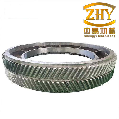
To overcome these inherent limitations, this study focuses on the manufacturing of recess-free herringbone gears using multi-axis CNC machining technology. By utilizing the flank milling method with cylindrical end mills on a five-axis machining center, I successfully eliminated the need for the recess while maintaining high gear precision. Unlike traditional hobbing or grinding methods that require dedicated custom tooling, the proposed approach employs standard off-the-shelf end mills, which significantly reduces tooling costs and lead times. This advantage is particularly pronounced in small-batch production scenarios where gears of varying modules, tooth numbers, and pressure angles are required. Through systematic investigation of machining processes, tool path optimization using the constant scallop height method, and UG secondary development for automated tool path generation, I have developed a comprehensive manufacturing solution for high-precision recess-free herringbone gears.
1. NC Machining Program for Recess-Free Herringbone Gear
1.1 Three-Dimensional Modeling
As the foundation for the entire machining study, a precise three-dimensional model of the recess-free herringbone gear was first established. I employed the GC Toolbox functionality embedded in Siemens NX 10.0 software to accomplish this task efficiently. The GC Toolbox, specifically designed for Chinese national standards (GB), provides parametric gear modeling capabilities that significantly accelerate the design process. The primary geometric parameters of the herringbone gear investigated in this research are summarized in Table 1.1. These parameters were derived from an actual engineering design requirement for a heavy-duty marine transmission application.
| Parameter | Symbol | Value | Unit |
|---|---|---|---|
| Module | m | 16 | mm |
| Number of teeth | z | 30 | – |
| Addendum coefficient | ha* | 1.0 | – |
| Pressure angle | α | 20 | ° |
| Helix angle | β | 30 / −30 | ° |
| Clearance coefficient | c* | 0.25 | – |
The modeling procedure began by selecting the “Spur/Helical Gear” creation tool under the GC Toolbox menu. I input the module, number of teeth, pressure angle, and helix angle, and the software automatically generated a single helical gear body. Subsequently, the “Mirror Geometry” command was applied to create the mirrored helical gear section, thereby forming the complete herringbone gear geometry. The gear face width was established according to the design drawing, and the final three-dimensional model accurately represented the intended recess-free configuration.
1.2 Tool Selection and Machining Method Analysis
The selection of appropriate cutting tools is crucial for achieving both high machining quality and efficiency. For machining complex curved surfaces such as gear teeth, two primary types of tools are considered: ball-end mills and flat end mills. Ball-end mills offer the advantage of a constant cutting radius relative to the tool center, which simplifies tool path calculation for free-form surfaces. However, they exhibit significant drawbacks near the tool rotation center where cutting speed approaches zero, leading to poor surface finish and reduced tool life. Additionally, due to their geometrical characteristics, ball-end mills require smaller stepover distances, which extends machining time considerably.
In contrast, flat end mills distribute cutting edges along the cylindrical surface and are particularly effective for machining convex surfaces with relatively uniform curvature distribution. The involute tooth flank of a herringbone gear qualifies as such a surface. By employing the flank milling technique with a flat end mill, I achieved substantially larger machining stepover widths compared to ball-end milling, resulting in shorter tool paths and higher material removal rates. The fundamental cutting parameters for the flat end mills are derived from the following relationships:
The cutting speed is calculated as:
$$v_c = \frac{\pi d n}{1000}$$
where vc is the cutting speed (m/min), d is the cutter diameter (mm), and n is the spindle speed (r/min). The feed rate is determined by:
$$v_f = f \cdot n = f_z \cdot z_t \cdot n$$
where f is the feed per revolution (mm/r), fz is the feed per tooth (mm/z), and zt is the number of teeth on the cutter.
Based on the gear material requirements—which specified carburized and hardened surfaces with a hardness of HRC 58–62 and a core hardness of HRC 30–40—I selected PVD-coated solid carbide end mills. These tools offer an optimal balance between wear resistance, toughness, and cutting speed capability. The tool dimensions were determined by measuring the available space within the tooth space of the three-dimensional model. The measured minimum width at the tooth space bottom was 7.5373 mm, and the distance between the tops of the root fillet radii on both sides was 16.625 mm. Consequently, I established the following tool selection strategy:
- A ϕ20 mm carbide end mill for bulk material removal during rough machining of the tooth space above the pitch circle.
- A ϕ10 mm carbide end mill for rough machining of the narrower tooth space bottom region.
- A ϕ12 mm carbide end mill for semi-finishing and finishing operations of the tooth flanks.
- A ϕ8 mm carbide ball-end mill for semi-finishing and finishing of the root fillet areas.
The tool geometric parameters were carefully determined. A helix angle of 40° was selected for the ϕ20 mm end mill to facilitate effective chip evacuation, while a 30° helix angle was chosen for the ϕ12 mm end mill. A radial rake angle of 10° was adopted for machining steel workpieces, and clearance angles of 12° and 15° were set for roughing and finishing tools, respectively.
The machining parameters were established based on the workpiece material properties and tool characteristics. For roughing operations, a spindle speed range of 800–1200 r/min and a feed rate of 500 mm/min were selected. For semi-finishing and finishing operations, spindle speeds were increased to 2300–3000 r/min while maintaining the same feed rate. The complete machining process plan is presented in Table 1.2.
| Process | Operation type | Programming method | Tool type / mm | Spindle speed / r·min⁻¹ | Feed rate / mm·min⁻¹ |
|---|---|---|---|---|---|
| Rough slotting | Roughing | Variable-axis contour milling | ϕ20 end mill | 800–1200 | 500 |
| Rough milling of tooth space bottom | Roughing | Variable-axis contour milling | ϕ10 end mill | 800–1200 | 500 |
| Semi-finishing of tooth flank | Semi-finishing | Variable-axis contour milling | ϕ12 end mill | 2300–3000 | 500 |
| Semi-finishing of tooth space bottom | Semi-finishing | Variable-axis contour milling | ϕ10 end mill | 2300–3000 | 500 |
| Semi-finishing of root fillet | Semi-finishing | Variable-axis contour milling | ϕ8 ball-end mill | 2500 | 500 |
| Finishing of tooth flank | Finishing | Variable-axis contour milling | ϕ12 end mill, ϕ8 ball-end mill | 2500 | 500 |
1.3 NC Program Generation with UG CAM
The UG NX 10.0 CAM module provides a comprehensive suite of multi-axis machining capabilities that I utilized for generating the NC programs. The programming workflow, as illustrated in the schematic flow diagram, encompasses five main stages: process parameter definition, tool path generation, tool path editing, dynamic machining simulation, and post-processing. The “Variable Contour” command was selected as the primary programming method due to its exceptional versatility in handling complex sculptured surfaces, which perfectly aligns with the requirements of herringbone gear tooth flank machining.
In the initial setup phase, I established the machining coordinate system with the origin coinciding with the gear pitch circle center, and the gear face end plane aligned with the XOY plane. The raw material model was defined as a cylindrical blank with a diameter equal to the gear addendum circle diameter and a height corresponding to the total face width. A safe plane was set at a distance of 100 mm above the gear surface to ensure collision-free rapid positioning movements.
For the rough slotting operation, an auxiliary plane was created at the middle of the tooth space. A variable contour milling operation was configured with the “Surface” drive method, using the auxiliary plane as the driving geometry. The tool axis was controlled using the “4-axis relative to drive body” strategy, enabling the ϕ20 mm end mill to follow the helical tooth direction while maintaining proper tool orientation. The machining proceeded in a reciprocating cutting pattern, and the generated tool path is shown in Figure 2.2(a) with its corresponding 3D dynamic simulation result. After confirming the initial roughing path, I created a second roughing operation by copying the first one and modifying the surface drive parameters. Specifically, the “Start Step” percentage was adjusted from 60% to 95%, effectively reducing the area coverage to target the narrower region near the tooth space bottom, where the ϕ20 mm end mill would cause interference.
For the semi-finishing operation of the tooth flanks, the driving surface was changed to the actual tooth flank geometry. A key parameter adjustment involved setting the “Offset” value in the Surface Region Drive Method dialog. This offset created a uniform machining allowance of 1 mm on the tooth flank surface in preparation for the subsequent finishing operation. Similarly, the tooth space bottom semi-finishing operation employed the ϕ10 mm end mill with the same offset strategy, ensuring a consistent finishing allowance.
The finishing operations differed from the semi-finishing operations in two critical aspects. First, the cutting mode was changed from “Reciprocating” to “One-Way” to implement conventional milling, which provides better surface quality for finishing applications. Second, the offset value was set to zero, eliminating the machining allowance and ensuring that the cutting tool exactly traced the design surface profile. Figure 2.4 illustrates the finishing tool path for the tooth flank, and the 3D simulation of the root fillet finishing operation is presented in Figure 2.5. After completing the tool path generation for all operations, I performed comprehensive 3D dynamic simulations to verify that no interference or over-cutting would occur during the actual machining process.
2. Optimization of Flank Finishing Tool Path Based on Constant Scallop Height Method
2.1 Theoretical Foundations
The tooth flank of a herringbone gear is an involute helicoid surface, characterized by curvature that continuously varies along the involute profile. Specifically, the radius of curvature increases progressively from the involute start circle to the addendum circle. At the start circle, the radius of curvature attains its minimum value, while at the addendum circle, it reaches the maximum. This significant curvature variation has a direct impact on the permissible tool path stepover distance, which is the spacing between adjacent tool paths.
For a general curved surface being machined, the relationship between the stepover distance l, the surface radius of curvature r, and the scallop height λ can be expressed as:
$$l = \sqrt{8r\lambda – 4\lambda^2} \approx \sqrt{8r\lambda}$$
where the approximation is valid when the scallop height is substantially smaller than the radius of curvature—a condition that holds true for precision gear finishing operations. This relationship reveals that for a constant scallop height, the stepover distance increases with the square root of the radius of curvature. Therefore, when machining a surface with varying curvature, using a constant stepover distance derived from the minimum radius will inevitably result in smaller-than-necessary scallop heights (and thus redundant tool paths) in regions with larger curvature radii.
To quantitatively assess this phenomenon for the herringbone gear under investigation, I calculated the radii of curvature at both extremes of the involute profile. The radius of curvature at the involute start circle was determined to be 77.366 mm, while that at the addendum circle was 143.821 mm. Using a target scallop height of λ = 0.0025 mm—necessary to achieve the required Grade 6 precision—I computed the corresponding stepover distances. The MATLAB analysis results, depicted conceptually in Fig. 3.2, clearly demonstrate the nonlinear relationship among these three variables.
| Interval number | Stepover distance l |
|---|---|
| Interval 1 | 1.6864 |
| Interval 3 | 1.6499 |
| Interval 6 | 1.5908 |
| Interval 10 | 1.5063 |
| Interval 14 | 1.4094 |
| Interval 18 | 1.2989 |
| Interval 20 | 1.2346 |
The computed stepover distances ranged from approximately 1.2 mm at the involute start circle to approximately 1.7 mm at the addendum circle. This substantial variation of over 40% clearly indicates that conventional tool path planning methods-uniform-parameter or uniform-stepover strategies-would unavoidably generates redundant tool paths and waste significant machining time. Therefore, the constant scallop height method was deemed essential for this application.
2.2 Involute Helical Surface Equation
To establish a rigorous mathematical foundation for the machining analysis, I derived the parametric equations of the involute helical surface. The involute curve in its parametric form is expressed as:
$$\begin{cases} x = r_b(\cos\varphi + \varphi\sin\varphi) \\ y = r_b(\sin\varphi – \varphi\cos\varphi) \\ z = 0 \end{cases}$$
where rb is the base circle radius and φ is the pressure angle parameter. When this curve undergoes helical motion with lead h, the generated helical surface can be described through the composed transformation of the involute equation with the helical motion equations. The resulting involute helicoid parametric equation is:
$$\begin{cases} x = r_b[\cos(\varphi+\mu) + \varphi\sin(\varphi+\mu)] \\ y = r_b[\sin(\varphi+\mu) – \varphi\cos(\varphi+\mu)] \\ z = \frac{h}{2\pi}\mu \end{cases}$$
where μ is the helical motion parameter. When the parameter φ is held constant, these equations represent different helical lines on the surface. Conversely, when μ is constant, they represent different involute curves at various axial positions. The local helix angle at any point on the surface can be determined from:
$$\tan\beta = \frac{2\pi r}{h}$$
where r is the radial distance from the gear axis to that point on the helical line. This equation confirms that points at different radial distances possess different helix angles for the same lead, which is a critical consideration for generating accurate tool paths.
2.3 Tool Path Generation Strategy Using Constant Scallop Height
Based on the theoretical analysis above, I developed a specialized strategy for generating constant scallop height tool paths specifically for flank milling of the gear tooth surface. The key to this strategy is the derivation of the scallop height function that describes the relationship between adjacent tool paths when using a cylindrical end mill in flank milling.
As shown in the schematic diagram, when the end mill traverses along a given tool path, the cylindrical cutting surface generates a swept surface. The intersection of two adjacent swept surfaces must lie exactly on the offset surface of the designed tooth flank at the specified scallop height λ. When this condition is satisfied, the stepover distance achieves its maximum allowable value, thereby minimizing the number of tool paths without compromising surface quality.
For the actual implementation, I considered the tooth profile curve g(x). An auxiliary curve f(x) is defined as the offset of g(x) along its normal direction by the scallop height distance λ:
$$f(x) = g(x) – \lambda \mathbf{n}(x)$$
where n(x) is the unit normal vector at point x. By solving the system of equations between the offset curve f(x) and the tangent line through the next candidate point, the contact points are sequentially determined. The tangent point coordinates are found by solving:
$$\frac{dy_c}{dx} = \frac{y_c – y_{i+1}}{x_c – x_{i+1}}$$
This procedure starts from the initial contact point A (the intersection of the involute with the addendum circle), iteratively calculates each subsequent contact point along the involute toward the start circle, and terminates when the radial coordinate falls below the start circle radius r0. The complete contact point set was computed using a MATLAB program that I developed for this specific purpose.
| Item | Value |
|---|---|
| Number of tool paths (constant scallop height) | 21 |
| Number of tool paths (constant parameter) | 25 |
| Reduced tool paths | 4 per tooth flank |
| Scallop height value | 0.0025 mm |
| Number of gears teeth | 30 |
The calculation results indicated that the constant scallop height method required 21 tool paths to cover the entire tooth flank, whereas the conventional constant-parameter method necessitated 25 tool paths for the same region. This represents a reduction of 4 tool paths per tooth flank. Since the herringbone gear has 30 teeth and each tooth has two flanks (left-hand and right-hand), the total savings are substantial. If the machining time for a single tool path is denoted as t, the total time saved for machining one complete herringbone gear is:
$$T = 4 \cdot t \cdot z$$
where z = 30 is the number of teeth. This calculation quantitatively confirms the efficiency advantage of the constant scallop height approach.
3. Secondary Development of Tool Path Generation Program
3.1 Programming Preparation and Menu Design
The implementation of the constant scallop height tool path generation involves a complex sequence of calculations and geometric operations. Manually performing these steps for each gear would be extremely tedious and error-prone. Therefore, I undertook a secondary development project on the UG NX 10.0 platform to automate the entire process. The development environment was configured by creating a dedicated folder structure within the Siemens NX installation directory, comprising a “startup” subfolder for menu customization and an “application” subfolder for storing the application programs. An environment variable was also added to enable UG to locate the secondary development files.
Using UG/Open MenuScript, I designed a custom menu item that appears in the UG main menu bar. The menu creation involved writing a “.men” file with the appropriate version declaration matching UG NX 10.0. A label “Herringbone Gear Constant Scallop Height Finishing” was defined, and an action command was linked to the corresponding “.dfa” file that would be called when the menu item is selected. The menu was positioned to appear immediately after the UG Help menu for optimal visibility and accessibility.
3.2 Development Approaches
Two fundamentally different approaches were considered for the implementation of the tool path generation program:
Method I: Solid Modeling Approach. This method utilizes 3D modeling operations directly within UG. The procedure involves: (1) selecting the edge of the tooth flank at the addendum circle as the initial tool contact path; (2) creating a plane tangent to the tooth flank along this edge; (3) generating an offset surface of the tooth flank by the scallop height distance using the “Offset Surface” command; (4) determining the intersection curve between the tangent plane and the offset surface; and (5) repeating steps (2)–(4) to generate all subsequent tool contact paths. This approach leverages UG commands such as new_ug_offset_sheet_body for surface offsetting and new_ug_curve_intersection for curve intersection calculations. While conceptually straightforward, this method is only suitable for spur gears because the helical nature of the herringbone gear tooth lines complicates the tangent plane construction.
Method II: Point-Line Approach. This method involves a series of calculations in the two-dimensional domain first to determine the tool contact points, followed by the construction of three-dimensional tool paths from these points. The procedure starts with computing all the constant scallop height contact points along the involute profile using the iterative mathematical procedure described earlier. After obtaining the contact point set, each point is offset along the involute normal direction by the tool radius to obtain the tool center points. Finally, helical lines are constructed through these offset points to form the complete tool paths. The helix angle for each point is calculated based on the point’s radial distance and the gear’s lead using Eq. 10. This method was selected for the present development due to its applicability to both spur and helical gear configurations.
3.3 UI Interface Design and Implementation
The UI interface was designed using UG/Open UIStyler, incorporating a user-friendly layout with three distinct groups. The first group, “Tool Contact Point Selection,” enables the user to select the pre-computed contact points that have been imported into UG. The second group, “Parameter Settings,” provides numeric input fields for critical parameters including the base circle radius rb, helix angle β, contact point radius rx, and lead h. The third group, “Schematic Diagram,” displays an illustrative figure that helps the user understand the program’s functionality.
The UI implementation utilized several key programming constructs in the KF language. The selection component was created using the %ui_comp_selection command with appropriate filtering constraints to allow only single-face selection. Numeric input fields were implemented using %ui_comp_expression commands with expression variables bound to the parameter fields. The schematic image was embedded as a bitmap file using %ui_comp_label. The helical line generation algorithm was implemented using a for loop in the KF program, calling the ug_spline_thru command to construct spline curves through the generated points. Figure 4.9 presents the completed UI interface for both development methods, showing the distinct design layouts.
3.4 Tool Contact Point Calculation
The critical component of the entire secondary development is the accurate computation of constant scallop height tool contact points. I developed a MATLAB program to perform this iterative calculation with high precision. The algorithm operates as follows:
- Start from the initial contact point A(x0, y0) on the addendum circle.
- Compute the tangent line to the involute at A.
- Search for a new point B(x1, y1) on the involute such that the vertical distance between the tangent lines at A and B equals the prescribed scallop height λ.
- If the radial coordinate of point B satisfies x1² + y1² ≤ r0², terminate the iteration; otherwise, proceed to the next iteration.
The computed contact point coordinates for the analyzed herringbone gear are illustrated conceptually in Fig. 4.7. These coordinates were then imported into UG software where the point-line method program generated the helical tool contact paths. The final constant scallop height tool paths were obtained by offsetting these paths by the tool radius in the direction normal to the tooth flank surface. The generated tool paths demonstrated uniform scallop height distribution and minimal redundancy, thereby achieving the optimization objectives.
4. Machining Simulation and Experimentation
4.1 VERICUT Simulation Setup
Before conducting actual machining experiments, I performed comprehensive simulations using VERICUT software to verify the correctness of the NC programs and to compare the machining efficiency of different tool path strategies. The simulation environment replicated the actual machining conditions, encompassing the machining center model, tool assemblies, tool holders, and workholding fixtures. The following steps were undertaken:
The machine tool model was built based on the specifications of a DMU 210FD turn-mill center. This machining center features a working table diameter of 1850 mm, a maximum machining diameter of 2100 mm, and X/Y/Z axis travel ranges that accommodate the herringbone gear blank comfortably. The machine’s positioning accuracy and repeatability specifications are summarized in Table 4.1 for reference.
| Parameter | Value | Unit |
|---|---|---|
| Working table diameter | 1850 | mm |
| Max. machining diameter | 2100 | mm |
| X-axis positioning accuracy | 0.012 | mm |
| Y-axis positioning accuracy | 0.009 | mm |
| Z-axis positioning accuracy | 0.009 | mm |
| C-axis positioning accuracy | 7 | arcsec |
| X-axis repeatability | 0.007 | mm |
| Y-axis repeatability | 0.005 | mm |
| Z-axis repeatability | 0.005 | mm |
| C-axis repeatability | 5 | arcsec |
The cutting tools were modeled in VERICUT using the tool management module. Three tool assemblies were created: a ϕ20 mm end mill with a 26 mm flute length and 92 mm total length, a ϕ12 mm end mill with a 26 mm flute length and 83 mm total length, and a ϕ8 mm ball-end mill with a 16 mm flute length and 100 mm total length. Tool holders were modeled as a combination of a conical section and two cylindrical sections with appropriate dimensions, as shown in Figure 5.3(b). The workholding fixture was designed as a cylindrical component with dimensions of 480 mm diameter and 450 mm height, assembled to the machine table with its rotational center aligned to the table’s center.
4.2 Simulation Results and Efficiency Comparison
After completing the simulation setup, the NC programs generated from UG were imported into VERICUT and executed sequentially. The simulation ran successfully without any reported interference, over-cutting, or axis travel violations, confirming the correctness of the generated NC codes. The simulation also provided a systematic comparison of machining times between the two tool path strategies.
| Machining method | Simulated time per tooth | Actual time per tooth |
|---|---|---|
| Constant-parameter method | 48.73 | 63.0 |
| Constant-scallop-height method | 38.00 | 51.2 |
The simulation results demonstrated that the constant scallop height method requires 38 minutes to machine a single tooth flank, compared to 48.73 minutes for the constant-parameter method. This represents a 22% reduction in machining time for the finishing operation. The slight discrepancy between simulated and actual machining times can be attributed to tool inspection, operator interventions, and other practical factors during the real machining process.
A broader comparison between the proposed CNC machining approach and traditional hobbing-grinding methods is provided in Table 4.3. While the traditional method achieves a somewhat shorter overall machining time due to the use of specialized machinery and dedicated tooling, the preparation time involved in custom tool manufacturing (ranging from 20 days to 2 months) makes the CNC approach far more advantageous for small-batch production of gears with varying specifications.
| Machining method | Total machining time | Tooling preparation time |
|---|---|---|
| Proposed CNC method | 80 | Off-the-shelf tools |
| Traditional method | 50 | 20–60 days (custom tools) |
4.3 Machining Experiment
With the simulation results providing confidence in the process, I proceeded with the actual machining experiment on the DMU 210FD turn-mill center. The experimental setup included the following components:
A custom-designed workholding fixture was manufactured to secure the gear blank during machining. The fixture consisted of a base plate mounted to the machine table using clamping bolts, a locating spigot for radial positioning, and a keyed interface to prevent rotational movement. Two parallel keyways were machined on the fixture and the gear blank mating surfaces, enabling the insertion of a rectangular key (10 mm × 36 mm × 8 mm) to accurately restrict the rotational degree of freedom. This special connection was chosen over a simple friction clamp to ensure positive kinematic locking of the workpiece.
After mounting the gear blank with 45# steel, I executed the following procedure: (1) using the machine’s touch probe system to measure the blank’s rotation center and verifying that the outer diameter runout was within 0.01 mm; (2) starting the roughing program while monitoring the cutting noise and vibration; (3) periodically inspecting the tool condition for wear after each tooth slot; (4) transitioning to the semi-finishing program once all tooth spaces were roughed; and (5) executing the final finishing program with both constant-parameter and constant-scallop-height tool paths on different tooth flanks to allow direct comparison under identical machining conditions.
The machining parameters during the finishing phase were maintained at a spindle speed of 2500 r/min and a feed rate of 500 mm/min, consistent with the simulation parameters. During the finishing operation, I used a stopwatch to measure the actual machining time for each tooth flank, with the results recorded in Table 4.2. The experimental measurements confirmed that the constant scallop height method saved approximately 11.8 minutes per tooth compared to the constant-parameter method. For the complete herringbone gear with 30 teeth, this translates to a total time savings of 5 hours and 54 minutes, representing approximately 19% of the finishing time.
4.4 Measurement Results and Analysis
Following the completion of machining, the recess-free herringbone gear was measured using a Gleason 1500GMS gear inspection machine. This instrument employs a comparison measuring principle, where the actual gear is measured against a mathematically perfect gear model generated from the entered parameters. The measurement procedure involved mounting the gear on the inspection machine, generating the reference gear model, aligning the coordinate systems, and performing automatic measurement cycles for all tooth flanks.
The measurement results for the key gear accuracy parameters are presented in Table 4.4. All six measured parameters achieved the requirements of Grade 6 precision according to the Chinese National Standard (GB/T 10095). The maximum total profile deviation Fα was 11.3 μm, well below the allowable 23 μm. Similarly, the maximum total helix deviation Fβ was 11.5 μm, corresponding to the Grade 6 limit of 18 μm.
| Parameter | Max value | Min value | Average | Grade 6 limit |
|---|---|---|---|---|
| Total profile deviation, Fα | 11.3 | 7.6 | 9.7 | 23 |
| Profile form deviation, ffα | 9.2 | 3.8 | 5.8 | 18 |
| Profile slope deviation, fHα | 10.0 | 5.7 | 7.6 | ±15 |
| Total helix deviation, Fβ | 11.5 | 10.3 | 10.8 | 18 |
| Helix form deviation, ffβ | 3.3 | 2.6 | 3.0 | 13 |
| Helix slope deviation, fHβ | 11.7 | 10.5 | 11.1 | ±13 |
Analysis of the measurement report reveals several noteworthy observations. The helix slope deviations exhibit a consistent directional pattern across all measured teeth, suggesting a systematic error source. I identified three potential contributing factors: (1) the precision of the helical line modeling during the tool path generation, where small deviations in the spline construction could translate to consistent helix angle errors; (2) minor clearance in the keyed fixture connection, which could allow slight rotational movement of the workpiece under cutting forces; and (3) the inherent geometric error accumulation during the machining process. To mitigate these issues in future manufacturing runs, I propose the following improvements:
- Enhancing the accuracy of the helical line modeling in the KF program by using a finer discretization density for the spline construction.
- Replacing the keyed fixture connection with a hydraulic clamping system to eliminate clearance-induced positioning errors.
- Implementing periodic tool inspection and replacement at shorter intervals to minimize the effects of tool wear on the machined surface geometry.
- Optimizing the cutting parameters (particularly the spindle speed and feed rate selection) to reduce the risk of machining chatter.
5. Conclusions and Future Perspectives
This research has systematically addressed the challenge of manufacturing high-precision recess-free herringbone gears using advanced CNC machining technology. Through the integration of multiple technical approaches, I have achieved the following principal accomplishments:
First, a comprehensive machining process plan was designed specifically for recess-free herringbone gears. The plan utilizes standard flat end mills for flank milling operations, effectively eliminating the requirement for the traditional recess groove while maintaining excellent machining accuracy. The process encompasses roughing, semi-finishing, and finishing stages with carefully selected tool geometries and cutting parameters. This approach demonstrates superior flexibility for small-batch production of herringbone gears with varying specifications, significantly reducing both tooling costs and lead times compared to conventional methods.
Second, the constant scallop height method was successfully adapted and applied to the flank finishing of herringbone gear teeth. Through rigorous mathematical derivation of the involute helical surface equations and the stepover distance relationships, I established a systematic procedure for generating evenly distributed tool paths with maximum allowable stepover distances. The implementation on the actual gear with 16 mm module and 30 teeth resulted in a reduction of tool paths from 25 to 21 per tooth flank, corresponding to a 19% reduction in finishing time. The simulated and experimentally verified time savings of approximately 5 hours and 54 minutes per gear demonstrates the substantial economic benefit of this optimization.
Third, a semi-automated tool path generation program was developed through UG NX secondary development. The program provides a user-friendly interface featuring tool contact point selection, parameter input, and visual guidance. The point-line method approach ensures applicability to both spur and helical gears, extending the program’s utility beyond the specific herringbone gear investigated in this study. The KF programming language facilitated the modular implementation of the helical line generation algorithm.
Fourth, the entire machining process was verified through both computational simulation and actual machining experiments. VERICUT simulation confirmed the absence of interference and over-cutting issues, while the machining trials on a DMU 210FD turn-mill center successfully produced the gear with all measured parameters meeting Grade 6 precision requirements. The measurement results, with maximum profile deviation of 11.3 μm and helix deviation of 11.5 μm, strongly validated the effectiveness of the proposed manufacturing methodology.
Looking forward, several avenues for future research and development can be identified. The tool axis vector orientation during ball-end milling of the root fillet regions presents an optimization opportunity—special attention should be paid to avoiding the low-cutting-speed zone near the ball-end mill’s rotation center. The feasibility of combining climb and conventional milling regimes in a single finishing pass deserves investigation, as this could potentially further reduce machining time, although the impact on surface quality requires careful evaluation. Additionally, the extension of the constant scallop height method to handle tooth flank modifications such as profile crowning or helix crowning would broaden the applicability of this approach. These ongoing research directions will further enhance the industrial applicability and efficiency of recess-free herringbone gear manufacturing.
In conclusion, this research has demonstrated that recess-free herringbone gears can be manufactured to high precision using standard end mills on multi-axis CNC machines, achieving optimal machining efficiency through the constant scallop height method and automated tool path generation. The comprehensive engineering solution developed herein provides a solid foundation for the broader adoption of herringbone gears in compact, high-performance transmission systems where traditional recess-machining constraints have previously imposed significant design limitations.