
1. Introduction and Research Background
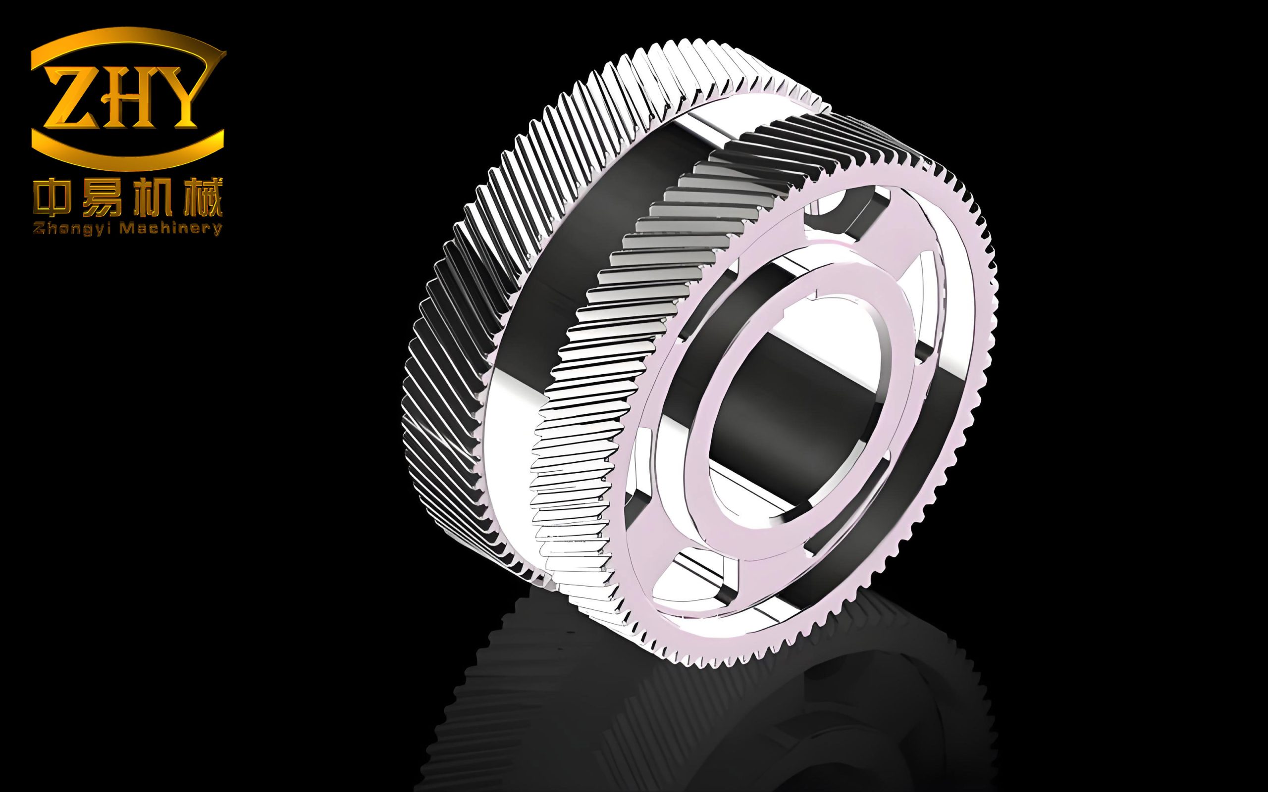
High-speed herringbone gear transmission systems are widely applied in energy, petrochemical, aerospace, and marine propulsion sectors due to their exceptional load-carrying capacity, smooth torque transmission, and reduced axial thrust compared to single-helical gears. The unique double-helical configuration of the herringbone gear inherently balances axial forces, making it particularly suitable for high-power-density applications. However, as modern machinery continues to advance toward higher rotational speeds, greater power densities, and more stringent reliability requirements, the dynamic performance of these gear systems has become a critical bottleneck. During high-speed operation, the herringbone gear system is subjected to complex internal excitations—including time-varying mesh stiffness, transmission errors, tooth side clearance, and gear mesh impacts—along with external excitations such as unbalanced rotor forces and bearing oil film forces. These multi-source excitations can induce severe vibrations and noise, threatening operational stability and safety.
In engineering practice, the manufacturing, assembly, and operating processes inevitably introduce substantial uncertainties in geometric parameters, material properties, and loading conditions. Traditional deterministic optimization approaches fail to account for these uncertainties, often leading to designs that perform well nominally but exhibit significant performance degradation or premature failure in real-world applications. Therefore, robust optimization design that systematically considers uncertainty has become increasingly important.
This study focuses on developing a comprehensive methodology for the dynamic performance optimization of high-speed herringbone gear transmission systems. The research encompasses four major aspects: (1) dynamic excitation characterization; (2) flexible multi-body dynamics modeling and vibration analysis; (3) six-sigma robust optimization design; and (4) experimental validation on a prototype gearbox. Throughout this work, I systematically investigate the vibration generation mechanisms, establish accurate simulation models, propose effective resonance identification criteria, and implement robust optimization methods to reduce vibration while maintaining structural integrity.
2. Dynamic Excitation Characterization of Herringbone Gear Transmission
Accurate characterization of internal dynamic excitations is fundamental to gear dynamics analysis. In this section, I present the computational methods for time-varying mesh stiffness, transmission error, backlash, and bearing support parameters of the herringbone gear pair.
2.1 Gear Pair Configuration and Basic Parameters
The high-speed single-stage herringbone gear transmission system studied in this work consists of a pinion and gear both manufactured with double-helical teeth. The basic geometric parameters of the gear pair are summarized in the following table:
| Parameter | Symbol | High-Speed Gear | Low-Speed Gear |
|---|---|---|---|
| Number of teeth | z | 92 | 46 |
| Module (mm) | m | 7 | 7 |
| Normal pressure angle (°) | αn | 25 | 25 |
| Face width (mm) | b | 30 | 30 |
| Helix angle (°) | β | 23.38 | 23.38 |
| Density (kg/m³) | ρ | 7850 | 7850 |
| Elastic modulus (Pa) | E | 2.1×10¹¹ | 2.1×10¹¹ |
| Poisson’s ratio | ν | 0.3 | 0.3 |
| Center distance (mm) | a | 530±0.0315 | — |
2.2 Contact Line Length Analysis
Unlike spur gears, the herringbone gear pair engages gradually along the tooth width direction. The instantaneous contact line length on the plane of action varies periodically with the rotation angle. Based on the geometry of the contact zone shown in Figure 2-2 of the original analysis, I define the base pitch in the transverse plane as pbt and the total contact ratio-related length Lε = εα·pbt. For the case where the face width remains smaller than the helical overlap length, the contact line length l(t) can be expressed piecewise as:
$$l(t) = \begin{cases} \frac{v_0 t}{\sin\beta_b}, & t \in [0, t_1] \\[6pt] \frac{B}{\cos\beta_b}, & t \in [t_1, t_2] \\[6pt] \frac{v_0 t \tan\beta_b + L_{\varepsilon} – v_0 t}{\sin\beta_b}, & t \in [t_2, t_3] \\[6pt] 0, & t \in [t_3, T_n] \end{cases}$$
where v₀ = π·n₁·rb1/30 is the rolling velocity of the contact line, n₁ and rb1 represent the rotational speed and base radius of the driving gear, respectively, εα is the transverse contact ratio, and Tn is the meshing period of a single tooth pair. The gradual engagement characteristic of the herringbone gear results in substantially reduced mesh impact compared to spur gears, contributing to smoother dynamic behavior.
2.3 Time-Varying Mesh Stiffness Calculation
Time-varying mesh stiffness (TVMS) constitutes the primary internal excitation in gear systems. I employ the potential energy method combined with the slicing approach to calculate the TVMS of the herringbone gear pair. The total potential energy stored in a meshing tooth pair consists of four components: Hertzian contact energy Uh, bending energy Ub, shear deformation energy Us, and axial compression energy Ua. Consequently, the corresponding stiffness components are determined as:
$$k_h = \frac{F^2}{2U_h}, \quad k_b = \frac{F^2}{2U_b}, \quad k_s = \frac{F^2}{2U_s}, \quad k_a = \frac{F^2}{2U_a}$$
Considering the gear tooth as a non-uniform cantilever beam, the bending stiffness for a slice of thickness ΔL along the face width is expressed as:
$$k_b = \sum_{i=1}^{N} \frac{1}{\int_{-\alpha_1′}^{\alpha_2} \frac{3\left[1+\cos\alpha_1′(\alpha_2-\alpha)\cos\alpha – \cos\alpha_1’\right]^2}{2E\left(\sin\alpha + (\alpha_2-\alpha)\cos\alpha\right)^3} \, d\alpha} \cdot \Delta L$$
where N is the number of slices along the tooth width, and α₁’ accounts for the angular position of the contact point. Similarly, the shear stiffness and axial compressive stiffness can be formulated as:
$$k_s = \sum_{i=1}^{N} \frac{1}{\int_{-\alpha_1′}^{\alpha_2} \frac{1.2(1+\nu)(\alpha_2-\alpha)\cos\alpha \cos^2\alpha_1′}{\sin\alpha + (\alpha_2-\alpha)\cos\alpha} \, d\alpha} \cdot \Delta L$$
$$k_a = \sum_{i=1}^{N} \frac{1}{\int_{-\alpha_1′}^{\alpha_2} \frac{(\alpha_2-\alpha)\cos\alpha \sin^2\alpha_1′}{2\left(\sin\alpha + (\alpha_2-\alpha)\cos\alpha\right)} \, d\alpha} \cdot \Delta L$$
The foundation flexibility stiffness kf is determined from the gear body deformation model:
$$\delta_f = \frac{F\cos^2\alpha}{WE} \left[ L^*\left(\frac{u_f}{S_f}\right)^2 + M^*\left(\frac{u_f}{S_f}\right) + P^*(1 + Q^*\tan^2\alpha) \right]$$
where the polynomial coefficients L*, M*, P*, and Q* are functions of the geometric parameters hfi and θf. The single-tooth-pair mesh stiffness is then obtained as:
$$\frac{1}{k_e} = \frac{1}{k_{b1}} + \frac{1}{k_{s1}} + \frac{1}{k_{a1}} + \frac{1}{k_{f1}} + \frac{1}{k_{b2}} + \frac{1}{k_{s2}} + \frac{1}{k_{a2}} + \frac{1}{k_{f2}} + \frac{1}{k_h}$$
For the case of multiple tooth pairs in simultaneous contact, the total mesh stiffness is computed by summing the contributions of each engaging pair:
$$k = \sum_{j=1}^{n} \frac{1}{\frac{1}{k_{h,j}} + \frac{1}{k_{b1,j}} + \frac{1}{k_{s1,j}} + \frac{1}{k_{a1,j}} + \frac{1}{k_{f1,j}} + \frac{1}{k_{b2,j}} + \frac{1}{k_{s2,j}} + \frac{1}{k_{a2,j}} + \frac{1}{k_{f2,j}}}$$
To validate the analytical solution, I established a finite element model of the herringbone gear pair using ANSYS. The teeth were modeled with refined hexahedral mesh elements, and surface-to-surface contact elements with a friction coefficient of 0.05 were applied. By constraining the high-speed gear and applying torque to the low-speed gear, the angular deformation was extracted to compute the mesh stiffness. The comparison between the analytical method and the finite element method is shown in the following table:
| Method | Average mesh stiffness (N/m) | Computational time | Accuracy |
|---|---|---|---|
| Analytical (energy method) | 2.72×10⁷ | Seconds | Reference |
| Finite element method | 2.68×10⁷ | Hours | Deviation < 1.5% |
The results demonstrate that the analytical energy method provides mesh stiffness values very close to those from high-fidelity finite element analysis while dramatically reducing computational cost. This efficiency is essential for iterative design optimization tasks requiring numerous evaluations.
2.4 Transmission Error Modeling
Manufacturing and assembly errors cause deviations from the ideal meshing position. The static transmission error can be expressed as a superposition of harmonic components related to the rotational frequency and mesh frequency:
$$e(t) = 0.5F_{p} \sin(\omega_r t + \phi_r’) + 0.5F_{p}’ \sin(\omega_m t + \phi_m’)$$
where Fp is the cumulative pitch deviation, Fp‘ is the composite deviation including pitch and profile deviations, ωr is the rotational frequency of the gear, ωm is the mesh frequency, and φr‘, φm‘ are the initial phase angles. For the high-speed gear with cumulative pitch deviation Fp = 0.034 mm and the low-speed gear with Fp = 0.044 mm, the transmission error varies periodically at both shaft rotation and tooth meshing frequencies, contributing broadband excitation to the system.
2.5 Tooth Side Backlash
Backlash is necessary for proper lubrication, thermal expansion accommodation, and smooth operation of gear pairs. The backlash function g(δ) is piecewise defined as:
$$g(\delta) = \begin{cases} \delta – b, & \delta > b \\[4pt] 0, & -b \le \delta \le b \\[4pt] \delta + b, & \delta < -b \end{cases}$$
where b represents half of the normal backlash and δ is the relative displacement along the line of action. The minimum backlash is calculated using the empirical relationship:
$$2b_{min} = \frac{2}{3}(0.06 + 0.0005a + 0.03m)$$
This backlash nonlinearity introduces a softening characteristic that can significantly affect the dynamic response at light loads and during speed transients.
2.6 Bearing Support Stiffness and Damping
The herringbone gear system studied in this work utilizes journal bearings as rotor supports. I employed the DyRoBeS software package to compute the bearing dynamic coefficients. The bearing geometry consists of a cylindrical bore with a length-to-diameter ratio chosen for optimal stability. The computed stiffness and damping matrices for the high-speed and low-speed bearings are:
| Bearing | Stiffness (N/mm) | Damping (N·s/mm) |
|---|---|---|
| HS Bearing 1-2 | kxx=5.859×10⁵, kxy=1.194×10⁵, kyx=-1.093×10⁵, kyy=8.763×10⁵ | cxx=1.015×10³, cxy=-7.841×10², cyx=-7.841×10², cyy=3.259×10³ |
| LS Bearing 3-4 | kxx=6.968×10⁵, kxy=-1.480×10⁵, kyx=-8.701×10⁵, kyy=5.709×10⁵ | cxx=1.849×10³, cxy=-1.714×10², cyx=-1.714×10², cyy=3.241×10³ |
The cross-coupled stiffness coefficients reflect the oil film hydrodynamic effects, which play a significant role in the rotordynamic stability of high-speed gear systems.
3. Dynamic Modeling and Vibration Analysis
3.1 Flexible Multi-Body Dynamics Theory
For accurate dynamic analysis of the high-speed herringbone gear system, I adopted a flexible multi-body dynamics approach. The generalized coordinates of a flexible body consist of Cartesian coordinates x, y, z, Euler angles ψ, θ, φ, and modal coordinates q. The position vector of an arbitrary point on the flexible body is:
$$\mathbf{r}_p = \mathbf{x} + \mathbf{A}(\mathbf{s}_p + \boldsymbol{\phi}_p \mathbf{q})$$
where A is the transformation matrix, sp is the undeformed position, and φp is the modal matrix of translational degrees of freedom. The equations of motion of the flexible multi-body system are given by:
$$\mathbf{M}\ddot{\mathbf{q}} + \mathbf{D}\dot{\mathbf{q}} + \mathbf{K}\mathbf{q} + \frac{\partial \mathbf{C}}{\partial \mathbf{q}}^T \boldsymbol{\lambda} = \mathbf{F}_a + \mathbf{F}_g$$
where M, D, and K are the mass, damping, and stiffness matrices, respectively; C represents the constraint equations; λ is the Lagrange multiplier vector; Fa is the applied external force vector; and Fg is the generalized gravitational force.
3.2 Finite Element Model Development
I constructed a comprehensive three-dimensional finite element model of the gearbox system, consisting of the gear housing, high-speed shaft with gear, low-speed shaft with gear, and four journal bearings. The gearbox housing was discretized using SOLID185 elements with refined hexahedral meshing for the gears and shafts, while tetrahedral elements were used for complex housing geometries. The journal bearings were modeled using COMBIN14 spring-damper elements with stiffness and damping values from the DyRoBeS calculations. The complete model comprises 700,954 nodes and 400,116 elements.
| Component | Material | Density (kg/m³) | Elastic Modulus (Pa) | Poisson’s Ratio |
|---|---|---|---|---|
| Gears | Alloy steel | 7870 | 2.1×10¹¹ | 0.30 |
| Shafts | Alloy steel | 7850 | 2.1×10¹¹ | 0.31 |
| Housing | Cast iron | 7850 | 2.1×10¹¹ | 0.33 |
3.3 Modal Analysis Results
Modal analysis of the gearbox system was performed using the Block Lanczos method. The first eight natural frequencies and their associated vibration modes are listed below:
| Mode | Frequency (Hz) | Dominant Vibration Mode |
|---|---|---|
| 1 | 131.16 | Gear shaft torsion with housing sway along Y-axis |
| 2 | 164.98 | First-order bending of low-speed shaft with housing sway along X-axis |
| 3 | 202.49 | Housing extension/compression along Z-axis |
| 4 | 209.09 | Low-speed shaft bending with housing torsion about Z-axis |
| 5 | 238.18 | Low-speed shaft bending with housing base deformation |
| 6 | 282.47 | Housing base extension along Z-axis |
| 7 | 307.48 | Housing torsion with low-speed shaft bending |
| 8 | 316.59 | Housing base deformation about Z-axis |
The operating speed of 6000 r/min corresponds to a shaft rotational frequency of 100 Hz and a mesh frequency of 4600 Hz. The excitation frequencies are sufficiently separated from the first eight natural frequencies, suggesting that the gearbox will not experience resonance at the rated operating condition.
3.4 Critical Speed Analysis
I performed a Campbell diagram analysis to determine the critical speeds of the gear-shaft system. The rotational speed was varied from 0 to 40,000 r/min while computing the natural frequencies that vary with speed due to gyroscopic effects. The results indicate:
| Mode | Direction | Stability | Critical Speed (r/min) |
|---|---|---|---|
| 1 | Backward whirl | Stable | 13,062 |
| 2 | Forward whirl | Stable | 14,908 |
| 3 | Backward whirl | Stable | 29,598 |
| 4 | Backward whirl | Stable | 30,057 |
| 5 | Backward whirl | Stable | 36,286 |
The first critical speed is 14,908 r/min, which is more than twice the rated speed of 6,000 r/min. This provides an adequate safety margin, ensuring stable operation across the intended speed range.
3.5 Potential Resonance Point Identification
I proposed a systematic three-principle methodology for identifying potential resonance points within the operating speed range:
(1) Frequency Principle: Considering the excitation frequency upper limit as six times the high-speed shaft rotational frequency or three times the mesh frequency, I selected 600 Hz as the frequency ceiling. This includes the first 36 modes of the system.
(2) Damping Principle: Modes with damping ratios outside the under-damped range (0 < ζ < 1) were excluded. The first six modes exhibited critical damping (ζ = 1), representing rigid-body motions, and were eliminated from further consideration.
(3) Energy Principle: For each remaining mode, I computed the modal energy distribution across all six degrees of freedom. If the total rotational energy (about α, β, and γ axes) was less than unity, the mode was considered unlikely to be excited. The energy criterion can be expressed as:
$$E_{\alpha}^i + E_{\beta}^i + E_{\gamma}^i > 1$$
Applying these three principles successively, I screened the 36 computed modes down to one potential resonance point at 164.98 Hz (Mode 8). Since the operating frequency is 100 Hz, the system avoids resonance at rated conditions. However, this potential resonance frequency should be avoided during speed-up and coast-down transients.
3.6 Vibration Response Analysis
Using the mode superposition method, I calculated the steady-state vibration response of the gearbox system at various operating speeds. Four evaluation points were defined: Points 1 and 2 located at the mid-span of the input and output shafts, respectively, and Points 3 and 4 on the top surface of the gearbox housing directly above the high-speed and low-speed gear shafts.
The shaft vibration displacement results at different speeds are summarized:
| Speed (r/min) | Evaluation Point | Direction | Displacement (μm) |
|---|---|---|---|
| 3000 | 1 | X | 14.86 |
| Y | 13.97 | ||
| 2 | X | 6.10 | |
| Y | 5.50 | ||
| 4000 | 1 | X | 17.46 |
| Y | 15.57 | ||
| 2 | X | 7.48 | |
| Y | 6.68 | ||
| 5000 | 1 | X | 18.95 |
| Y | 18.71 | ||
| 2 | X | 12.11 | |
| Y | 10.34 | ||
| 6000 | 1 | X | 22.87 |
| Y | 20.27 | ||
| 2 | X | 15.32 | |
| Y | 13.63 |
The vibration displacement increases monotonically with rotational speed, consistent with the increased dynamic excitation at higher speeds. The input shaft exhibits larger vibrations than the output shaft, reflecting the higher torque transmission on the high-speed side.
At the rated speed of 6000 r/min, the housing vibration acceleration levels at evaluation points 3 and 4 were calculated:
| Evaluation Point | Direction | Acceleration (mm/s²) |
|---|---|---|
| 3 | X | 5881.5 |
| Y | 4408.2 | |
| Z | 4285.9 | |
| 4 | X | 5778.4 |
| Y | 5439.7 | |
| Z | 3923.1 |
The frequency domain analysis revealed that the vibration spectra exhibit dominant peaks at the gear mesh frequency (4600 Hz) and its sidebands, along with components at the shaft rotational frequency (100 Hz) and its harmonics.
4. Six-Sigma Robust Optimization Design
4.1 Robust Optimization Fundamentals
Robust design aims to minimize the influence of parameter variability on the system performance. The fundamental objectives include: (1) minimizing the variance of the quality characteristic, σ²y = E[(y − μy)²], and (2) reducing the deviation of the mean from the target value, δ²y = E[(μy − y₀)²]. This dual objective ensures that the performance not only meets the target but also remains consistent despite manufacturing tolerances and operational variations.
4.2 Design Variables and Optimization Model
I selected seven design variables related to the gearbox housing dimensions. These variables, their baseline values, ranges, and statistical distributions are:
| Variable | Description | Initial Value (mm) | Range (mm) | Distribution |
|---|---|---|---|---|
| x₁ | Housing cover thickness | 14 | 9–19 | Normal |
| x₂ | Housing wall thickness | 24 | 19–29 | Normal |
| x₃ | Housing base plate thickness | 14 | 9–19 | Normal |
| x₄ | Reinforcement rib thickness | 10 | 5–15 | Normal |
| x₅ | Block thickness | 24 | 19–29 | Normal |
| x₆ | Inner support plate thickness | 24 | 19–29 | Normal |
| x₇ | Crossbeam dimension | 90 | 80–100 | Normal |
The six-sigma robust optimization problem is formulated as:
$$\text{Minimize} \quad F\left(\mu_f(\mathbf{x}), \sigma_f(\mathbf{x})\right) = w_1 \frac{\mu_f(\mathbf{x}) – f_0}{M_1} + w_2 \frac{\sigma_f(\mathbf{x})}{M_2}$$
Subject to the constraints:
$$G_i\left(\mu_f(\mathbf{x}), \sigma_f(\mathbf{x})\right) \le 0$$
$$x_{i,L} + 6\sigma_i \le x_i \le x_{i,U} – 6\sigma_i \quad i = 1, 2, \ldots, 7$$
$$V(\mathbf{x}) \le V_0$$
where μf(x) and σf(x) are the mean and standard deviation of the objective function (housing vibration acceleration), w₁ and w₂ are weighting factors, M₁ and M₂ are normalization constants, f₀ is the target value, and V₀ = 0.8917 m³ is the initial housing volume.
4.3 Sensitivity Analysis
Latin Hypercube Sampling (LHS) was employed to generate 20 sample points across the design space. The sensitivity analysis results revealed that the reinforcement rib thickness (x₄) and the housing base plate thickness (x₃) exert the most significant influence on the housing vibration acceleration response, followed by the housing cover thickness (x₁). A goodness-of-fit curve confirmed the accuracy of the response surface approximation, with sampled points clustering closely along the diagonal line.
4.4 Kriging Response Surface Modeling
To enable efficient statistical analysis within the six-sigma framework, I constructed Kriging surrogate models to approximate the relationship between design variables and vibration responses. Kriging interpolation combines a global polynomial trend function with local deviations, providing an exact interpolation at sample points while quantifying prediction uncertainty. The Kriging predictor takes the form:
$$\hat{y}(\mathbf{x}) = \mathbf{f}(\mathbf{x})^T \boldsymbol{\beta} + \mathbf{r}(\mathbf{x})^T \mathbf{R}^{-1}(\mathbf{Y} – \mathbf{F}\boldsymbol{\beta})$$
where f(x) is the trend function vector, β is the regression coefficient vector, r(x) is the correlation vector between a new point and the sample points, R is the correlation matrix, Y is the vector of observed responses, and F is the design matrix. The response surface analysis demonstrated that the housing vibration acceleration exhibits relatively flat regions within the design space, indicating opportunities for robust optimization.
4.5 Optimization Results
The six-sigma robust optimization yielded the following optimal design parameters:
| Variable | Initial Value (mm) | Optimal Value (mm) | Rounded Value (mm) | Change (%) |
|---|---|---|---|---|
| x₁ | 14 | 12.4857 | 12 | -14.3 |
| x₂ | 24 | 22.1458 | 22 | -8.3 |
| x₃ | 14 | 15.4265 | 15 | +7.1 |
| x₄ | 10 | 11.3906 | 11 | +10.0 |
| x₅ | 24 | 27.3374 | 27 | +12.5 |
| x₆ | 24 | 20.2262 | 20 | -16.7 |
| x₇ | 90 | 80.2657 | 80 | -11.1 |
The optimized design achieved a total housing mass reduction of 58.712 kg while simultaneously improving dynamic performance. The vibration acceleration responses at the evaluation points were significantly reduced after optimization:
| Evaluation Point | Direction | Before Optimization (mm/s²) | After Optimization (mm/s²) | Reduction (%) |
|---|---|---|---|---|
| 3 | X | 5881.5 | 3224.2 | 45.2 |
| Y | 4408.2 | 2908.3 | 33.7 | |
| Z | 4285.9 | 2901.5 | 30.4 | |
| 4 | X | 5778.4 | 3312.7 | 42.6 |
| Y | 5439.7 | 3205.4 | 41.1 | |
| Z | 3923.1 | 2899.6 | 26.1 |
4.6 Robustness Assessment
I evaluated the reliability and sigma levels for the key design variables after optimization. For the housing base plate thickness of 15.4265 mm, the reliability reached 98.6%; for the reinforcement rib thickness of 11.3903 mm, the reliability was 99.7%; and for the housing cover thickness of 12.4857 mm, the reliability was 97.2%. The probability density functions of these critical variables shifted toward the target values while maintaining narrow distributions, confirming that the optimal design achieves both performance improvement and robustness to parameter variations.
5. Experimental Validation
5.1 Test Rig Configuration
Based on the optimized design, I fabricated a prototype high-speed herringbone gearbox and constructed a comprehensive performance test platform. The test rig layout consisted of a drive motor, torque sensor, speed-increasing gearbox, and the test gearbox, all connected via flexible couplings. The test system was configured to measure shaft vibration displacement, housing vibration acceleration, temperature rise, power consumption, and noise levels.
Eddy current proximity probes were installed at the input and output shaft bearing locations, positioned at 45° angles to the horizontal and vertical axes, defining the X and Y measurement channels with a probe gap of 1 mm. Four tri-axial accelerometers were mounted on the gearbox housing top surface, each located 20 cm from the side walls directly above the gear shaft centerlines. A data acquisition system using NI-9231 and NI-9215 modules in a cDAQ chassis recorded all vibration signals at a sampling rate of 15,000 Hz.
5.2 Test Procedure
The test protocol included: (1) lubrication system stabilization at 130,000 Pa oil pressure; (2) progressive speed ramp from 500 r/min to 3000 r/min to check for abnormal noise or vibration; (3) sustained operation at 6000 r/min for one hour with bearing temperature monitoring; (4) overspeed test at 6600 r/min for 20 minutes; (5) steady-state measurement at each test speed, maintaining operation for 2 minutes before recording 30 seconds of data; and (6) long-duration thermal stability test at 6000 r/min for 2 hours with temperature logging every 5 minutes.
5.3 Shaft Vibration Displacement Results
The measured shaft vibration displacement values at various speeds are:
| Speed (r/min) | Point 1 X (μm) | Point 1 Y (μm) | Point 2 X (μm) | Point 2 Y (μm) |
|---|---|---|---|---|
| 3000 | 12.56 | 11.57 | 4.77 | 4.49 |
| 4000 | 13.73 | 13.56 | 5.04 | 4.54 |
| 5000 | 16.43 | 15.73 | 8.51 | 8.19 |
| 6000 | 19.10 | 17.50 | 9.46 | 8.67 |
At the rated speed of 6000 r/min, the maximum radial shaft vibration displacement was measured at 19.1 μm, which is well below the typical acceptance limit for high-speed gearboxes. The vibration waveforms exhibited predominantly synchronous components corresponding to the rotational frequency, with minimal sub-synchronous activity, indicating stable bearing operation.
5.4 Housing Vibration Acceleration Results
The measured housing acceleration root-mean-square (RMS) values at 6000 r/min are compared with simulation predictions:
| Evaluation Point | Direction | Experimental (m/s²) | Simulation (m/s²) | Deviation (%) |
|---|---|---|---|---|
| 3 | X | 3.187 | 3.224 | 1.2 |
| Y | 2.811 | 2.908 | 3.4 | |
| Z | 2.098 | 2.902 | 27.7 | |
| 4 | X | 2.776 | 3.313 | 16.2 |
| Y | 2.491 | 3.205 | 22.3 | |
| Z | 1.807 | 2.900 | 37.7 |
The experimental values generally show good agreement with simulation in the X and Y directions, with deviations within acceptable engineering tolerances. The larger discrepancies in the Z direction suggest that the simplified connection model between the housing and the test rig base affects the vertical vibration transmission, a factor not fully captured in the simulation model.
5.5 Temperature Rise Test
At the rated speed of 6000 r/min, the steady-state temperatures were recorded as follows: oil inlet temperature of 46.5°C, oil outlet temperature of 58.3°C, low-speed shaft input bearing at 54.8°C, low-speed shaft output bearing at 56.8°C, high-speed shaft input bearing at 53.4°C, and high-speed shaft output bearing at 48.5°C, with an ambient temperature of 29°C. The maximum temperature rise of approximately 29°C is well within the acceptable limit for mineral oil lubricated journal bearings.
5.6 Power Consumption Test
I measured the power consumption at various operating speeds:
| Speed (r/min) | Input Torque (N·m) | Power Loss (kW) | Loss Ratio (%) |
|---|---|---|---|
| 500 | 44 | 2.3 | 0.01 |
| 1200 | 89 | 11.2 | 0.06 |
| 3000 | 222 | 69.6 | 0.35 |
| 5400 | 338 | 191.5 | 0.96 |
| 6000 | 362 | 227.2 | 1.14 |
The single-stage transmission efficiency at rated speed was calculated as 98.86%, exceeding the design requirement of 98.5%. The power loss shows the expected quadratic relationship with rotational speed, consistent with viscous-dominated losses in the journal bearings and gear mesh.
5.7 Noise Measurement
At a distance of 1 meter from the gearbox operating at 6000 r/min, the noise levels at three measurement positions were: 111.7 dB(A), 106.5 dB(A), and 109.5 dB(A). These values are comparable to those of similar high-speed gearboxes in industrial applications and are primarily dominated by mesh frequency components and aerodynamic noise from the rotating gears.
6. Conclusions and Future Perspectives
This research presented a systematic methodology for the dynamic characterization, analysis, and robust optimization of high-speed herringbone gear transmission systems. The key contributions and findings of this work are summarized as follows:
(1) I established an analytical framework for dynamic excitation characterization of high-speed herringbone gear pairs, including time-varying mesh stiffness calculation using the energy method with the slicing technique. The analytical results agreed closely with finite element predictions while offering superior computational efficiency. I also characterized transmission error, tooth backlash, and bearing support stiffness and damping, providing comprehensive excitation inputs for dynamic analysis.
(2) I developed a flexible multi-body dynamic model of the complete gearbox system and performed modal analysis, critical speed analysis, and vibration response predictions. The proposed resonance identification principles—frequency, damping, and energy criteria—provided a systematic and effective method for screening potential harmful resonance points in the operating speed range. The gear shaft system exhibited its first critical speed at 14,908 r/min, providing a comfortable margin above the rated speed of 6,000 r/min.
(3) I implemented a six-sigma robust optimization methodology for the gearbox housing, considering seven geometric design variables with statistical distributions. The optimized design achieved simultaneous improvements in vibration reduction (26–45% reduction across different directions and evaluation points) and mass reduction (58.7 kg). The reliability analysis confirmed that the optimal design maintains robust performance despite parameter variability, with reliability levels exceeding 97% for the most critical variables.
(4) I fabricated and tested a prototype optimized gearbox, validating the simulation predictions. At the rated speed of 6,000 r/min, the maximum shaft vibration displacement was 19.1 μm, the transmission efficiency reached 98.86%, and the temperature rise remained within acceptable limits. The successful experimental validation confirms the effectiveness of the proposed dynamic optimization methodology for high-speed herringbone gear transmission systems.
Several directions merit further investigation in future work. The current dynamic model assumes ideal gear geometry apart from the measured transmission errors; incorporating tooth surface modifications (profile and lead crowning) would improve prediction accuracy. The effects of thermo-elastic deformation on gear meshing at high speeds should be investigated. In the optimization framework, additional uncertainty sources—such as varying operational loads, temperature-dependent material properties, and bearing clearance tolerances—should be incorporated. Finally, the application of multi-objective Bayesian optimization with active learning could further enhance the computational efficiency of the robust design process for larger-scale gear transmission systems.