
1. Introduction
During my postgraduate research, I focused on the dynamic characteristics of herringbone gear transmission systems incorporating friction excitation. A herringbone gear, also known as a double-helical gear, consists of two oppositely inclined helical gear halves on a single gear blank. This configuration offers significant advantages over spur and helical gears, including higher load-carrying capacity, negligible axial thrust, and smoother meshing behavior. These attributes make herringbone gears particularly suitable for high-speed and heavy-duty applications in aerospace, marine propulsion, and industrial power transmission.
Friction excitation is ubiquitous in mechanical transmission systems. It has been estimated that approximately one-third of the world’s primary energy consumption is dissipated through friction, and more than half of mechanical component failures are related to friction and wear. In gear transmissions, tooth surface friction significantly influences the dynamic behavior, vibration characteristics, and overall reliability of the system. Despite the critical role of friction, many dynamic analyses of herringbone gear transmissions have traditionally neglected this factor. Therefore, investigating the dynamic response of herringbone gear systems with friction excitation is of considerable academic and practical importance.
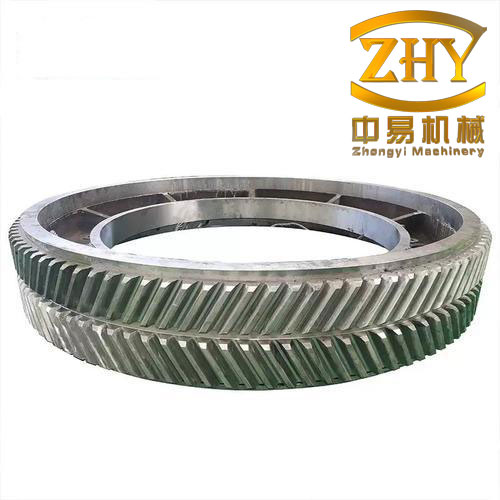
My research aims to develop a comprehensive dynamic model for herringbone gear transmissions, incorporating friction excitation, and to analyze the effects of various factors such as centering error and tooth tip modification. The key contributions of this work include a novel time-varying contact line length calculation method that accounts for friction-induced complexities, a systematic comparison of dynamic responses with and without friction, and a detailed analysis of manufacturing and modification influences on system behavior.
2. Research Significance and Objectives
The significance of this research lies in the pursuit of higher reliability, greater power density, and improved efficiency in gear transmission systems. As modern machinery demands increasingly complex operating conditions, the dynamic performance of herringbone gears becomes a limiting factor in overall system performance. Specifically, my objectives are:
- To establish a frictionless dynamic model of herringbone gear transmission and analyze its inherent dynamic characteristics.
- To extend the model to incorporate time-varying friction excitation and investigate its impact on gear dynamic responses.
- To analyze the influence of centering error on the dynamic behavior of herringbone gear transmission with friction.
- To evaluate the effects of tooth tip modification on the dynamic response of the friction-inclusive system.
3. Frictionless Herringbone Gear Dynamics
3.1 Modeling Approach
For the dynamic modeling of herringbone gear systems, I adopted a lumped-parameter approach. The herringbone gear pair is equivalent to two identical helical gear pairs operating in parallel, which simplifies the geometric complexity while preserving essential dynamic characteristics. The dynamic model considers the gear bodies as rigid masses with elastic tooth meshing interfaces, supported by flexible bearings and shafts.
I established a 12-degree-of-freedom (DOF) bending-torsion coupling dynamic model in a spatial coordinate system. Two coordinate systems were considered: a global coordinate system and a relative coordinate system. In the relative coordinate system, I aligned the line-of-action direction such that the meshing force lies entirely within the YOZ plane, allowing the X-direction to be exclusively governed by friction effects. This clever coordinate arrangement significantly simplified the dynamic equations.
3.2 Excitation Sources in Gear Systems
Gear transmission systems are subjected to various excitation sources that can be broadly classified into internal and external excitations. In my research, the following internal excitations were considered:
| Excitation Type | Description | Modeling Approach |
|---|---|---|
| Stiffness Excitation | Time-varying mesh stiffness due to alternating number of tooth pairs in contact | ISO standard calculation based on contact line length |
| Friction Excitation | Tooth surface friction force varying with contact line length and sliding direction | Integral of friction coefficient × normal load over instantaneous contact line |
| Error Excitation | Static transmission error from manufacturing and assembly deviations | Simplified sinusoidal function approximation |
| Damping Excitation | Mesh damping and support damping affecting system energy dissipation | Rayleigh damping model with equivalent mesh damping calculation |
External excitations such as load torque fluctuations, unbalance, and external disturbances were not considered in the current model to isolate the effects of internal excitations.
3.3 Time-Varying Contact Line Length Analysis
The time-varying contact line length is a critical parameter governing both mesh stiffness and friction excitation. The herringbone gear parameters used in my analysis are given in Table 1.
| Parameter | Symbol | Value |
|---|---|---|
| Number of teeth (pinion) | Z1 | 37 |
| Number of teeth (gear) | Z2 | 79 |
| Module | m | 2.5 mm |
| Normal pressure angle | α | 20° |
| Helix angle | β | 15° |
| Face width | B | 25 mm |
Given these parameters, the transverse contact ratio is approximately εα = 1.8 and the axial contact ratio is approximately εβ = 1.2. The total contact ratio is therefore approximately εγ = 3.0, resulting in a three-pair and two-pair alternating meshing pattern during rotation.
For a single tooth pair, the contact line length varies as the gear rotates through the meshing zone. The single-tooth contact line length follows a trapezoidal profile, which can be mathematically expressed for the condition εα < εβ as:
$$l(t) = \begin{cases} k_b t, & 0 \leq t < t_1 \\ l_{max}, & t_1 \leq t < t_2 \\ l_{max} – k_b (t – t_2), & t_2 \leq t < t_3 \\ 0, & t \geq t_3 \end{cases}$$
where kb represents the rate of change of contact line length proportional to the base tangential velocity and helix angle effects, lmax is the maximum contact line length, and t1, t2, t3 are critical time instants determined by the geometry and kinematics of the meshing process.
The total contact line length for the herringbone gear is obtained by summing the contributions of all tooth pairs simultaneously in contact, accounting for the phase differences between adjacent teeth equal to one base pitch. I formulated a multi-segment piecewise function for the total contact line length, with segmentation points determined by the entry and exit events of each tooth in the meshing zone.
3.4 Dynamic Mesh Force Calculation
The time-varying mesh force is computed by integrating the elastic force per unit contact length over the total instantaneous contact line length. The mesh stiffness K(t) is expressed as:
Considering the single-tooth contact scenario with unit line load stiffness k₀, the total time-varying mesh stiffness can be calculated as:
$$K(t) = k_0 \cdot L_{total}(t)$$
where Ltotal(t) is the total time-varying contact line length. The mesh damping C(t) is similarly expressed as:
$$C(t) = c_0 \cdot L_{total}(t)$$
with c₀ being the equivalent damping coefficient per unit contact line length.
The dynamic mesh force F(t) is then given by:
$$F(t) = K(t) \cdot f(\delta(t)) + C(t) \cdot \dot{\delta}(t)$$
where δ(t) is the relative displacement at the meshing point incorporating both the dynamic transmission error and the gear tooth deflection, and f(δ) is a backlash function defined as:
$$f(\delta) = \begin{cases} \delta – \frac{b}{2}, & \delta > \frac{b}{2} \\ 0, & |\delta| \leq \frac{b}{2} \\ \delta + \frac{b}{2}, & \delta < -\frac{b}{2} \end{cases}$$
where b is the gear backlash. The relative displacement δ(t) accounts for the combined axial and tangential motion of the gear teeth along the line of action.
3.5 Dynamic Equations of the 12-DOF Model
Employing Newton’s second law, I derived the 12-degree-of-freedom dynamic equilibrium equations for the herringbone gear transmission system. For the pinion, denoted by subscript q, and the gear, denoted by subscript p, the equations for each degree of freedom (translational X, Y, Z and rotational) take the following form:
For the left-side pinion (subscript q1):
$$m_{q1}\ddot{x}_{q1} + c_{q1x}\dot{x}_{q1} + k_{q1x}x_{q1} = 0$$
$$m_{q1}\ddot{y}_{q1} + c_{q1y}\dot{y}_{q1} + k_{q1y}y_{q1} = -F_1$$
$$m_{q1}\ddot{z}_{q1} + c_{q1z}\dot{z}_{q1} + k_{q1z}z_{q1} = -F_1\tan\alpha_t$$
$$I_{q1}\ddot{\theta}_{q1} = T_{q1} – F_1 r_{b1}$$
Similarly, for the right-side pinion (subscript q2):
$$m_{q2}\ddot{x}_{q2} + c_{q2x}\dot{x}_{q2} + k_{q2x}x_{q2} = 0$$
$$m_{q2}\ddot{y}_{q2} + c_{q2y}\dot{y}_{q2} + k_{q2y}y_{q2} = -F_2$$
$$m_{q2}\ddot{z}_{q2} + c_{q2z}\dot{z}_{q2} + k_{q2z}z_{q2} = -F_2\tan\alpha_t$$
$$I_{q2}\ddot{\theta}_{q2} = T_{q1} – F_2 r_{b1}$$
For the left-side gear (subscript p1):
$$m_{p1}\ddot{x}_{p1} + c_{p1x}\dot{x}_{p1} + k_{p1x}x_{p1} = 0$$
$$m_{p1}\ddot{y}_{p1} + c_{p1y}\dot{y}_{p1} + k_{p1y}y_{p1} = F_1$$
$$m_{p1}\ddot{z}_{p1} + c_{p1z}\dot{z}_{p1} + k_{p1z}z_{p1} = F_1\tan\alpha_t$$
$$I_{p1}\ddot{\theta}_{p1} = -T_{p1} + F_1 r_{b2}$$
And for the right-side gear (subscript p2):
$$m_{p2}\ddot{x}_{p2} + c_{p2x}\dot{x}_{p2} + k_{p2x}x_{p2} = 0$$
$$m_{p2}\ddot{y}_{p2} + c_{p2y}\dot{y}_{p2} + k_{p2y}y_{p2} = F_2$$
$$m_{p2}\ddot{z}_{p2} + c_{p2z}\dot{z}_{p2} + k_{p2z}z_{p2} = F_2\tan\alpha_t$$
$$I_{p2}\ddot{\theta}_{p2} = -T_{p2} + F_2 r_{b2}$$
In the 12-DOF model, the translational degrees of freedom correspond to the X, Y, and Z directions at each node for pinion and gear, respectively. The torsional degrees of freedom are associated with θq1, θq2, θp1, and θp2. Given the assumption of identical left and right helical gear halves, the axial degrees of freedom are coupled through the shaft axial stiffness kqz and kpz.
3.6 Nondimensionalization and Solving Procedure
To improve computational efficiency and accuracy, I performed nondimensionalization of the dynamic equations by introducing a characteristic time scale ωn and a length scale bc (typically the backlash magnitude). The dimensionless variables are defined as:
$$\bar{t} = \omega_n t, \quad \bar{x} = \frac{x}{b_c}, \quad \bar{y} = \frac{y}{b_c}, \quad \bar{z} = \frac{z}{b_c}$$
Substituting these into the original equations yields a set of dimensionless ordinary differential equations, which are then reduced to first-order form by introducing velocity variables. I employed a fourth-order Runge-Kutta method implemented in MATLAB (ode45 function) with adaptive step-size control to solve the resulting system.
3.7 Simulation Results for Frictionless Case
I conducted numerical simulations at three rotational speeds: 600 rpm (low speed), 2000 rpm (medium speed), and 5000 rpm (high speed), with a constant input torque. The frictionless dynamic responses are summarized below.
| Speed | Mesh force behavior | Dynamic transmission error | Y-direction deformation | Z-direction deformation |
|---|---|---|---|---|
| 600 rpm | Piecewise linear variation, low amplitude fluctuation | Almost constant, negligible fluctuation | Minimal fluctuation | Minimal fluctuation |
| 2000 rpm | Curved variation, reduced peak amplitude | Moderate amplitude with periodic variation | Visible periodic variation | Visible periodic variation |
| 5000 rpm | Increased amplitude, phase shift in peaks | Largest amplitude, phase shift observed | Largest deformation amplitude | Largest deformation amplitude |
The frequency spectrum analysis revealed that the primary periodic component dominates the dynamic response at all speeds, with the secondary periodic component being most pronounced at 2000 rpm and least at 5000 rpm.
4. Herringbone Gear Dynamics with Friction
4.1 Time-Varying Contact Line Length on Both Sides of the Pitch Line
Friction excitation in gear meshing is characterized by a direction reversal at the pitch line. Therefore, it is essential to compute the time-varying contact line length separately for regions on both sides of the pitch line. I divided the contact zone into two regions: the approach region (left side of pitch point) with length lp and the recess region (right side of pitch point) with length lg. For each tooth pair, I derived piecewise functions for the contact line lengths in these two regions, a1 and a2, respectively.
For the specific gear parameters used in this study (εα < εβ and lp < εβPbt < lg), the contact line length on the left side of the pitch line is expressed as:
$$a_1(S) = \begin{cases} 0, & 0 \leq S < l_p \\ k_b(S – l_p), & l_p \leq S < l_p + \varepsilon_\beta P_{bt} \\ k_b \varepsilon_\beta P_{bt}, & l_p + \varepsilon_\beta P_{bt} \leq S < l_g \\ k_b(l_s – S), & l_g \leq S < l_s \\ 0, & S \geq l_s \end{cases}$$
Similarly, for the right side of the pitch line:
$$a_2(S) = \begin{cases} k_b S, & 0 \leq S < l_g – l_p \\ 0, & l_g – l_p \leq S < l_p \\ k_b(S – l_p), & l_p \leq S < l_g \\ k_b(l_s – S), & l_g \leq S < l_s \\ 0, & S \geq l_s \end{cases}$$
where S represents the distance traveled along the line of action, and ls = lp + lg is the total length of the contact path.
For the total time-varying contact line length on each side of the pitch line, I summed the contributions of all tooth pairs in contact during one mesh cycle, accounting for the phase shifts between adjacent teeth. This yielded a multi-segment piecewise function with up to nine distinct segments within one mesh cycle.
4.2 Time-Varying Friction Excitation Model
The tooth surface friction force is computed by integrating the product of friction coefficient and normal load density over the instantaneous contact line length, separately for each side of the pitch line. The net friction force is:
$$F_f(t) = \mu F_n(t) \left[ L_{left}(t) – L_{right}(t) \right]$$
where μ is the average friction coefficient, Fn(t) is the instantaneous normal mesh force per unit length, Lleft(t) and Lright(t) are the total contact line lengths on the left and right sides of the pitch line, respectively.
Similarly, the friction torque on the pinion is:
$$T_{fq} = \mu F_n(t) \left[ \sum_{i=1}^{N_1} R_{c1i} l_{1i}(t) – \sum_{j=1}^{N_2} R_{c2j} l_{2j}(t) \right]$$
where Rc1i and Rc2j are the moment arms (radii) for each contact segment, and l1i(t), l2j(t) are the corresponding segment lengths. The friction torque on the gear is analogously expressed with appropriate moment arms.
4.3 16-DOF Dynamic Model of Herringbone Gear with Friction
I extended the 12-DOF model to a 16-DOF model by incorporating additional degrees of freedom associated with friction-induced axial motion and the independent axial displacement of each gear body. The equations of motion for the pinion and gear now include the friction force components in the X-direction (the direction perpendicular to the YOZ plane):
$$m_{q1}\ddot{x}_{q1} + c_{q1x}\dot{x}_{q1} + k_{q1x}x_{q1} = -F_{f1}$$
$$m_{q2}\ddot{x}_{q2} + c_{q2x}\dot{x}_{q2} + k_{q2x}x_{q2} = -F_{f2}$$
$$m_{p1}\ddot{x}_{p1} + c_{p1x}\dot{x}_{p1} + k_{p1x}x_{p1} = F_{f1}$$
$$m_{p2}\ddot{x}_{p2} + c_{p2x}\dot{x}_{p2} + k_{p2x}x_{p2} = F_{f2}$$
The rotational equations are also modified to include the friction torque terms:
$$I_{q1}\ddot{\theta}_{q1} = T_{in} – F_1 r_{b1} – T_{fq1}$$
$$I_{p1}\ddot{\theta}_{p1} = -T_{out} + F_1 r_{b2} + T_{fp1}$$
where Tfq1 and Tfp1 denote the friction torques acting on the left-side pinion and gear, respectively. The mesh force F1 for the left side now includes the effects of relative displacement δ1 and its time derivative.
4.4 Numerical Results and Discussion
4.4.1 Time-Varying Mesh Force
The time-varying mesh force of the herringbone gear with friction excitation is presented in Figure 8. At low speeds, the force variation exhibits nearly piecewise linear characteristics. At medium speeds, the force variation becomes smoother and the peak amplitude decreases. At high speeds, the peak amplitude increases again, with slight phase shifts in the peak and valley positions.
| Speed | Frictionless peak force (N) | With friction peak force (N) | Relative difference |
|---|---|---|---|
| 600 rpm | 8547 | 8561 | 0.16% |
| 2000 rpm | 8132 | 8155 | 0.28% |
| 5000 rpm | 8864 | 8892 | 0.32% |
The comparison demonstrates that friction excitation has a negligible influence on the magnitude and phase of the time-varying mesh force. This is because the primary function of the mesh force is governed by the normal compliance at the tooth contact interface, which is dominated by the stiffness and damping characteristics rather than the tangential friction effects.
4.4.2 Dynamic Transmission Error
Similar to the mesh force, the dynamic transmission error exhibits negligible change due to friction excitation. The overall trend of the dynamic transmission error with speed is consistent with the frictionless case: increasing amplitude with increasing rotational speed, with low-speed operation showing almost constant transmission error.
4.4.3 Tooth Deformation Along the X-Axis (Friction-Dominated Direction)
Unlike the mesh force and transmission error, the tooth deformation in the X-axis direction is significantly influenced by friction excitation. This is clearly illustrated in the simulation results. With friction, the X-axis deformation exhibits pronounced periodic fluctuations that intensify with rotational speed. At low speeds (600 rpm), the X-axis deformation is small but observable, whereas at high speeds (5000 rpm), it demonstrates the largest amplitude variation among all cases considered.
The frequency content of the X-axis deformation with friction is richer at low speeds, with multiple frequency components visible. As speed increases, the frequency content concentrates on the primary mesh frequency.
The Y-axis and Z-axis deformations are also slightly modified by friction excitation. For the Y-axis, the deformation amplitude shows minor differences compared to the frictionless case. The Z-axis deformation is nearly unaffected in both amplitude and phase, suggesting that the principal influence of friction is confined to the X-axis direction, consistent with the model formulation.
4.4.4 Effect of Damping on Friction Dynamics
I also investigated the influence of damping excitation on the friction-inclusive dynamic responses. When all damping terms are set to zero, the system becomes highly unstable, with significant fluctuations in the mesh force and transmission error. The deformation responses no longer exhibit the regular periodic patterns observed in the damped system, with large-amplitude oscillations appearing at all speeds. This indicates that damping plays a crucial role in stabilizing the herringbone gear system when friction excitation is present.
5. Influence of Centering Error on Herringbone Gear Dynamics
5.1 Definition and Modeling of Centering Error
Centering error is a common manufacturing and assembly error in herringbone gears. It describes the offset between the midpoints of the left and right helical gear teeth along the axial direction. Mathematically, the centering error ΔT is defined as:
$$\Delta T = l_2 – l_1 = l_4 – l_3$$
where l₁ and l₂ represent the distances from the tooth surfaces of the left and right gears to a reference plane at the gear boundary, and l₃ and l₄ represent similar distances for the opposite tooth flanks.
| Centering Error (μm) | Application/Loading Condition | Observable Effects |
|---|---|---|
| 20 | Precision gearboxes, light to medium loading | Minor phase shift between left and right mesh forces |
| 50 | General industrial applications | Visible phase shift, slight increase in mesh force peak |
| 150 | Heavy-duty applications with manufacturing deviations | Notable force imbalance, increased fluctuation at peak |
| 250 | Severe misalignment or worn gears | Significant force imbalance, pronounced peak fluctuations |
| 500 | Extreme conditions / test validation | Large peak dips, distinct spectral content changes |
The centering error introduces a phase shift between the left and right helical gear halves, affecting the time-varying contact line lengths, mesh stiffness, and consequently the dynamic response.
5.2 Effect of Centering Error on Contact Line Length and Mesh Stiffness
The centering error does not alter the single-tooth contact line length characteristics of each helical gear half individually; rather, it induces a phase shift between the left and right halves. This phase shift modifies the instantaneous total contact line length distribution, which in turn affects the mesh stiffness.
Employing the ISO standard stiffness formulation given by:
$$K(t) = k_0 L_{total}(t)$$
with the mesh stiffness per unit length k₀ derived from the tooth flexibility, the centering error modifies Ltotal(t) in the region around peak engagement, where the left and right halves are simultaneously contributing.
5.3 Dynamic Response of Herringbone Gear with Centering Error
I simulated the dynamic response of the herringbone gear transmission with a centering error of ΔT = 50 μm under the operating conditions used previously. Figure 11 shows the time-varying mesh force with centering error, while Figure 14 and 15 present the X-direction and Y-direction deformations.
From the obtained results, the following observations can be made:
- The centering error induces a phase lead in the right-side gear relative to the left-side gear, which is consistent with the assumed positive centering error sign.
- The dynamic transmission error increases slightly due to the centering error, potentially attributed to the phase difference-induced load redistribution.
- For the tooth deformations along the X, Y, and Z axes, the most significant effect of centering error is introducing a phase shift between the left and right gear responses. The amplitude of the deformation of the right-side gear (which enters the meshing zone earlier) exhibits larger fluctuations.
- Friction excitation, modulated by both the mesh force and the contact line distribution, is likewise amplified by the centering error, which could increase system vibration and noise.
5.4 Quantification of Centering Error Influence on Total Mesh Force
A systematic parametric study was performed for centering errors spanning from 25 μm to 500 μm, with the following key indicators evaluated:
| Centering Error (μm) | αt (% base pitch) | Maximum mesh force (N) | βFM (%) | Peak minimum force (N) | βFMI (%) |
|---|---|---|---|---|---|
| 0 | 0 | 10420 | 0.00 | 10420 | 0.00 |
| 25 | 4.2 | 10431 | 0.11 | 10134 | -2.74 |
| 50 | 8.4 | 10445 | 0.24 | 9850 | -5.47 |
| 100 | 16.8 | 10462 | 0.40 | 9310 | -10.65 |
| 150 | 25.2 | 10478 | 0.56 | 8770 | -15.83 |
| 200 | 33.7 | 10495 | 0.72 | 8230 | -21.02 |
| 250 | 42.1 | 10510 | 0.86 | 7690 | -26.20 |
| 400 | 67.4 | 10532 | 1.08 | 6550 | -37.14 |
| 500 | 84.2 | 10540 | 1.15 | 5840 | -43.95 |
The analysis reveals two distinct effects of centering error:
- Maximum mesh force: The maximum value of the total mesh force remains nearly constant, increasing by only about 1% even for large centering errors up to 500 μm. This indicates that the overall load-carrying capacity of the herringbone gear pair is not compromised by centering error alone.
- Peak stability: The mesh force in the vicinity of the peak value exhibits significant dips, and the magnitude of this dip increases approximately linearly with the centering error. This “valley” within the peak region suggests a transient unloading effect when the teeth of opposite helical halves cease to overlap their maximum contact lengths simultaneously.
6. Effect of Tooth Tip Modification on Herringbone Gear Dynamics
6.1 Tooth Tip Modification Concept
Tooth tip modification is a profile modification technique that selectively removes material from the tooth tip region to reduce mesh impact, vibration, and noise. It is defined by the maximum modification amount Δmax, the modification length (height) h, and the modification curve. The modification profile I used is parabolic:
$$e(x) = \Delta_{max} \left(\frac{x}{h}\right)^2$$
where x is the distance from the modification start point toward the tooth tip, e(x) is the modification amount at position x.
6.2 Time-Varying Mesh Stiffness of Modified Gear
I used a slicing method to calculate the mesh stiffness of the herringbone gear with tooth tip modification. The gear tooth is discretized into a number of thin slices, and the stiffness of each slice is computed using the formulation from Eq. (2) through (6). The individual slice stiffness values are then combined according to:
$$K_i = \begin{cases} 0, & \text{if } E_i – E_{min} > \varepsilon \\ \frac{k_{slice} \cdot F_n}{F_n + k_{slice} \cdot (E_i – E_{min})}, & \text{otherwise} \end{cases}$$
where Ei is the profile error/modification of the i-th slice, Emin is the minimum error among all active slices, ε is a tolerance threshold, kslice is the stiffness of the slice, and Fn is the nominal normal load. The total mesh stiffness is then the sum of all individual slice stiffness values.
| Modification height (mm) | Max modification (μm) | Mean mesh stiffness (N/m) | Stiffness fluctuation reduction (%) |
|---|---|---|---|
| 0 | 0 | 3.85 × 10⁸ | Baseline |
| 0.9 | 25 | 3.62 × 10⁸ | 17.4 |
| 1.2 | 25 | 3.48 × 10⁸ | 30.1 |
| 1.2 | 15 | 3.65 × 10⁸ | 21.3 |
| 1.2 | 5 | 3.79 × 10⁸ | 7.2 |
From Table 6, it is observed that increasing the modification height and maximum modification decreases the average mesh stiffness while simultaneously reducing the stiffness fluctuation—a key factor for vibration reduction in gear systems.
6.3 Dynamic Response of Modified Herringbone Gear
The time-varying mesh force for different modification profiles was computed at the same operating conditions (speed, torque) as for the unmodified gear. The key findings are:
- Mesh force smoothing: The time-varying mesh force of the modified gear exhibits a smoother variation profile with reduced abrupt changes, which enhances transmission smoothness and reduces dynamic loads.
- Frequency spectrum simplification: The mesh force frequency spectrum of the modified gear is simpler and has fewer higher-order harmonics, confirming improved dynamic behavior.
- Dynamic transmission error: The dynamic transmission error and tooth deformations along the X, Y, and Z axes are virtually unaffected by the modification at low speeds and low torques. This is because the concentrated-parameter model does not capture localized contact pressure variations that are more sensitive to modification. In real gears, however, modification improves load distribution and reduces peak pressures.
- Friction excitation: Since the friction force is proportional to both the normal load and the contact line length distribution, the reduction in mesh force amplitude and fluctuation with tooth tip modification leads to proportionally reduced friction excitation. This indirectly contributes to lowered vibration and enhanced system reliability.
7. Concluding Remarks
In this thesis, I have systematically investigated the dynamic characteristics of herringbone gear transmission systems with friction excitation. The following conclusions are drawn from my research:
- Frictionless dynamics: The 12-DOF lumped-parameter model effectively captures the dynamic behavior of a frictionless herringbone gear. The time-varying mesh force, dynamic transmission error, and bearing deformations show periodic fluctuations primarily at the mesh frequency, with amplitude increasing with rotational speed.
- Friction effects: The 16-DOF model incorporating friction excitation reveals that friction markedly affects the X-direction (perpendicular to the line-of-action direction) deformation responses, which are otherwise zero in a frictionless system. Friction induces additional vibration in this direction, with amplitude inversely related to shaft speed. Meanwhile, friction has a negligible effect on the mesh force and the dynamic transmission error.
- Damping interaction: System damping is crucial for the stability of friction-inclusive herringbone gear dynamics. In the absence of damping, the dynamic response becomes highly unstable, indicating strong coupling between friction and damping excitation.
- Centering error: The introduction of centering error induces a phase shift between the dynamic responses of the left and right gear halves. While the maximum total mesh force is hardly modified, the mesh force near the peak exhibits a dip whose depth increases nearly linearly with the centering error, potentially causing local unloading and subsequent impact. This also increases friction force fluctuation and system vibration.
- Tooth tip modification: Tooth tip modification reduces the mean mesh stiffness but also reduces stiffness fluctuation, leading to smoother mesh force variation and a simpler frequency spectrum. Modification length and maximum amount show a trade-off between stiffness reduction and dynamic smoothing, suggesting that optimal modification parameters should be selected based on operating conditions.
Future research directions include refining the mesh stiffness calculation using finite element methods, incorporating more realistic friction coefficient models based on elastohydrodynamic lubrication theory, and extending the analysis to multi-stage herringbone gear systems under varying external loads.
My work provides a theoretical foundation for the design optimization of herringbone gear transmissions in high-performance applications such as aerospace and marine power systems, and I hope it contributes meaningfully to the ongoing development of gear friction dynamics research.