
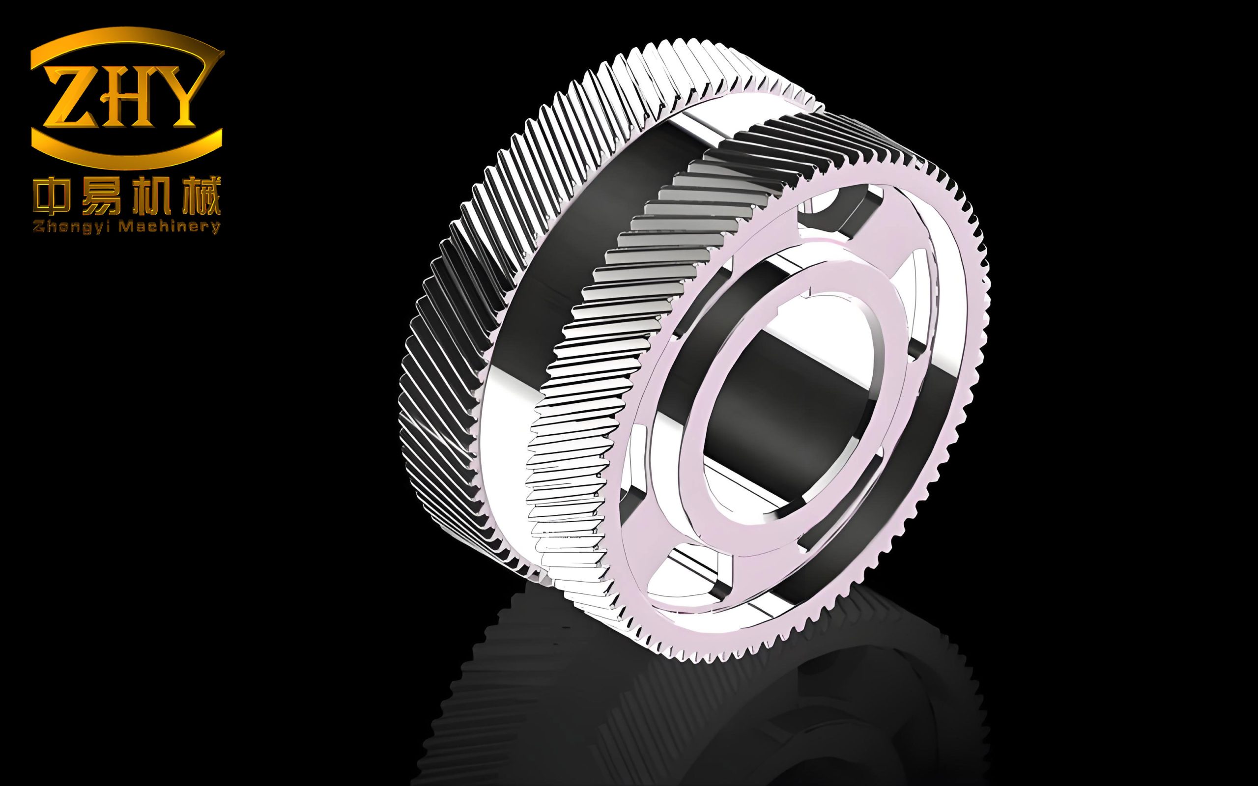
In my research, I focused on the prediction of time-varying meshing stiffness for herringbone gears considering manufacturing and assembly errors as well as tooth profile and lead modifications. Herringbone gears are widely used in high-speed and heavy-load transmission systems such as marine propulsion, aerospace reducers, and energy equipment because of their high contact ratio, zero net axial force, excellent load-sharing capacity, and smooth operation. The meshing stiffness is a key parameter for internal excitation and dynamic modeling of gear systems. It directly affects vibration, noise, and dynamic load distribution. Therefore, an accurate calculation method for the meshing stiffness of herringbone gears is essential for their design and optimization.
In this work, I first established an accurate three-dimensional geometric model of herringbone gears based on the generating principle. Then I built finite element models in ABAQUS and performed both static and dynamic contact analyses. I calculated the meshing stiffness using the finite element method and compared it with an analytical method. Furthermore, I investigated the effects of installation errors, misalignment errors, tooth profile modification, and lead crowning on the meshing stiffness. The results show that errors generally reduce the meshing stiffness, while appropriate modifications can improve the stiffness and load distribution.
1. Introduction
Herringbone gears are essentially two helical gears with opposite helix angles integrated into a single gear blank. They combine the advantages of helical gears while eliminating the axial thrust force. This makes them particularly suitable for heavy-duty applications such as main reducers in ships and helicopters. However, the complex tooth geometry and the presence of manufacturing and assembly errors complicate the accurate prediction of their meshing stiffness.
Many researchers have studied the dynamic behavior of gear systems, but most investigations focused on spur or helical gears. Only a limited number of studies have dealt with herringbone gear meshing stiffness. The main challenge lies in the fact that herringbone gears have a varying contact line length and multiple pairs of teeth in contact simultaneously. The total meshing stiffness is the sum of the stiffness of all contacting tooth pairs, and each pair contributes differently depending on the instantaneous contact position.
In my study, I employed the finite element method to compute the normal contact force and the comprehensive elastic deformation of the gear teeth. According to the basic definition of stiffness, I obtained the single-tooth stiffness, the single-pair meshing stiffness, and the total meshing stiffness. I also implemented an analytical approach based on the total contact line length and the stiffness per unit length. The comparison between the two methods verified the correctness of the finite element approach.
2. Finite Element Contact Analysis of Herringbone Gears
2.1 Geometric Modeling
To establish an accurate geometric model, I derived the tooth profile equation from the generating theory. The rack cutter and the workpiece satisfy the conjugate principle. I established three coordinate systems: a fixed coordinate system \(S(PXY)\), a movable coordinate system \(S_1(O_1X_1Y_1)\) attached to the rack, and another movable coordinate system \(S_2(O_2X_2Y_2)\) attached to the gear blank. The rack moves a distance \(s = r\varphi\), where \(r\) is the pitch radius and \(\varphi\) is the gear rotation angle. By applying the coordinate transformation matrix
$$
M_{21} =
\begin{bmatrix}
\cos\varphi & \sin\varphi & -r(\sin\varphi + \varphi\cos\varphi) \\
-\sin\varphi & \cos\varphi & -r(\cos\varphi – \varphi\sin\varphi) \\
0 & 0 & 1
\end{bmatrix},
$$
I obtained the general tooth profile equation of the gear:
$$
\begin{cases}
x_2 = (r + x_1)\cos\varphi + (r\varphi – y_1)\sin\varphi, \\
y_2 = (r + x_1)\sin\varphi – (r\varphi – y_1)\cos\varphi,
\end{cases}
$$
where \((x_1, y_1)\) are the coordinates of a point on the rack cutter profile.
For the tooth root transition curve, I considered the circular arc at the tip of the rack cutter. The coordinates of a point on this arc in the cutter coordinate system are
$$
\begin{cases}
x_1 = x_c + \rho \cos\gamma, \\
y_1 = y_c – \rho \sin\gamma,
\end{cases}
$$
where \(\rho\) is the radius of the tip arc, \(x_c\) and \(y_c\) are the center coordinates, and \(\gamma\) is the auxiliary angle. Substituting into the general equation yields the root transition curve expression.
For the involute portion, the rack cutter has a straight-sided tooth profile. The coordinates of a point on the straight flank are
$$
\begin{cases}
x_1 = r\varphi\sin\alpha + (y_0 – r\varphi)\cos\alpha, \\
y_1 = (y_0 – r\varphi)\sin\alpha,
\end{cases}
$$
where \(\alpha\) is the pressure angle and \(y_0\) is the offset distance. This leads to the involute profile equation in the gear coordinate system.
Since a herringbone gear is composed of two opposite helical gears, I derived the three-dimensional tooth surface equation by sweeping the end profile along the helix direction. For a helical gear with a helix angle \(\beta\), the tooth surface can be expressed as
$$
\begin{cases}
X = R(t)\cos\left(\dfrac{B\tan\beta}{r}t\right), \\
Y = R(t)\sin\left(\dfrac{B\tan\beta}{r}t\right), \\
Z = Bt,
\end{cases}
\quad 0 \le t \le 1,
$$
where \(R(t)=\sqrt{x_2^2+y_2^2}\), \(B\) is the tooth width, and \(r\) is the pitch radius. For the herringbone gear, the two halves are mirrored, so the tooth surface equation becomes
$$
\begin{cases}
X = R(t)\cos\left(\dfrac{B\tan\beta}{r}t\right), \\
Y = R(t)\sin\left(\dfrac{B\tan\beta}{r}t\right), \\
Z = \dfrac{B_w}{2} \pm Bt,
\end{cases}
$$
where \(B_w\) is the width of the central gap. I solved these equations using MATLAB to obtain discrete points on the tooth surface. Then I imported these points into CATIA and used surface fitting techniques to create a smooth geometric model. The basic parameters of the herringbone gear pair used in this study are listed in Table 1.
| Parameter | Pinion | Gear |
|---|---|---|
| Number of teeth \(z\) | 34 | 31 |
| Normal module \(m_n\) (mm) | 6 | |
| Normal pressure angle \(\alpha_n\) (°) | 25 | |
| Helix angle \(\beta\) (°) | 35.9891 | |
| Tooth width \(b_1\) (mm) | 180 | |
| Central gap width \(b_2\) (mm) | 24 | |
| Central gap depth \(d\) (mm) | 5.5 | 4 |
| Torque \(T\) (N·m) | 9545 | |
2.2 Finite Element Modeling
The herringbone gear geometry is complex, and direct structured meshing is difficult in ABAQUS. Therefore, I divided the gear body into individual teeth and then partitioned each tooth into eight hexahedral regions using auxiliary surfaces. The partitioning process is shown schematically in Figure 1. Each region was meshed with reduced-integration hexahedral elements (C3D8R). This element type provides good accuracy for contact problems while reducing computational cost. After meshing each region, I merged them to obtain a complete single-tooth mesh model, and then replicated it around the gear axis to form the full gear mesh model.
The material properties used in the finite element analysis are listed in Table 2. I used steel 45 with a Young’s modulus of 210 GPa and a Poisson’s ratio of 0.3.
| Material | Elastic modulus \(E\) (GPa) | Poisson’s ratio \(\mu\) | Density \(\rho\) (kg/m³) |
|---|---|---|---|
| Steel 45 | 210 | 0.3 | 7800 |
For static contact analysis, I defined a general static step. The gear was constrained by a reference point coupling technique: I created reference points on the axes of both gears and coupled them to the inner cylindrical surfaces of the gear bodies. This coupling allowed me to apply rotational boundary conditions to the gear. I fixed the pinion and applied a rotation angle to the gear, or vice versa, depending on which gear stiffness was being calculated.
For dynamic analysis, I used an explicit dynamic step. The input speed and torque were applied gradually to avoid numerical oscillations. Contact pairs were defined between the working flanks of the two gears. I considered both the drive side and the coast side to allow possible tooth disengagement and back-side contact at high speeds. The friction coefficient between the contacting surfaces was set to 0.06, which is typical for lubricated steel gears.
The static loading condition is given in Table 3. The dynamic loading conditions are given in Table 4. I selected speeds from 1000 to 10000 r/min to investigate the effect of rotational speed on the dynamic meshing characteristics under a constant torque of 9545 N·m.
| Case | Rotation angle (rad) | Torque (N·m) |
|---|---|---|
| Case 1 | 1.5 | 9545 |
| Case | Speed (r/min) | Torque (N·m) |
|---|---|---|
| Case 2 | 1000 | 9545 |
| Case 3 | 5000 | 9545 |
| Case 4 | 8000 | 9545 |
| Case 5 | 10000 | 9545 |
2.3 Static and Dynamic Contact Analysis
I first performed the static contact analysis to obtain the contact forces on the tooth flanks. From the finite element results, I extracted the normal contact force on a target tooth as a function of time. The contact force rose gradually during the approach, reached a maximum near the middle of the engagement, and then decreased to zero at the exit. By measuring the time difference between two successive tooth engagements and the total engagement time of a single tooth, I calculated the contact ratio as
$$
\varepsilon = \frac{\Delta T}{\Delta t}.
$$
For the standard gear pair without errors, the results showed \(\Delta T = 0.76\) s and \(\Delta t = 0.19\) s, giving \(\varepsilon = 4.0\). This high contact ratio is typical for herringbone gears and contributes to their smooth transmission.
The static analysis also provided the contact stress and bending stress distributions. The maximum contact stress was 364.9 MPa, and the maximum bending stress was 120.6 MPa. At the instant of tooth engagement, the contact stress was 484.9 MPa, and at disengagement it was 535.8 MPa. These relatively high values at the beginning and end of the mesh indicate the presence of mesh impact, but the overall meshing performance remained acceptable.
For the dynamic analyses, I obtained the rotational speeds of the pinion and gear for the four speed cases. The time required for the speeds to stabilize decreased as the rotational speed increased. At 1000 r/min, both gears ran smoothly. At 5000 r/min, the gear (driven) showed slight speed fluctuations. At 8000 and 10000 r/min, significant fluctuations appeared on the driven gear, and the contact force sometimes dropped to zero, indicating tooth separation and back-side contact. This phenomenon is more pronounced at higher speeds because the inertia forces overcome the elastic restoring forces.
The contact areas under dynamic conditions followed the same trend as the contact forces. The maximum contact area increased with speed. The contact stress and bending stress also increased with speed. Table 5 summarizes the maximum contact and bending stresses for all dynamic cases.
| Case | Maximum contact stress (MPa) | Maximum bending stress (MPa) |
|---|---|---|
| Case 2 (1000 r/min) | 877.2 | 289.3 |
| Case 3 (5000 r/min) | 2800.0 | 1574.6 |
| Case 4 (8000 r/min) | 5203.0 | 4803.0 |
| Case 5 (10000 r/min) | 6829.6 | 5468.9 |
These results demonstrate that herringbone gears are subject to severe impact loading at high rotational speeds. The dynamic stresses are much larger than the static values, which can lead to premature failure. Therefore, the design of high-speed herringbone gears must consider dynamic effects and appropriate modifications to reduce mesh impact.
3. Meshing Stiffness Calculation for Standard Herringbone Gears
3.1 Definition of Meshing Stiffness
The single-tooth stiffness of a gear is defined as the ratio of the normal contact force \(F_n\) to the comprehensive elastic deformation \(u_n\) at the contact point:
$$
K_n = \frac{F_n}{u_n}.
$$
The comprehensive elastic deformation includes the Hertzian contact deformation \(u_H\) and the bending deformation \(u_b\) at the tooth contact position:
$$
u_n = u_H + u_b.
$$
For a pair of gears in mesh, the single-pair meshing stiffness \(K\) is the series combination of the pinion stiffness \(K_1\) and the gear stiffness \(K_2\):
$$
K = \frac{K_1 K_2}{K_1 + K_2}.
$$
When multiple tooth pairs are simultaneously engaged, the total meshing stiffness is the parallel sum of the individual pair stiffnesses:
$$
K_{\text{total}} = \sum_{i=1}^{n} K_i,
$$
where \(n\) is the number of tooth pairs in contact.
3.2 Finite Element Calculation Procedure
I used the finite element method to compute the meshing stiffness of the herringbone gear pair. The finite element model is shown in Figure 2. To obtain the single-tooth stiffness of the pinion, I fixed the pinion and applied a torque to the gear while releasing its rotational degree of freedom. Similarly, to obtain the stiffness of the gear, I fixed the gear and applied a torque to the pinion. The target tooth was selected, and its contact stress distribution was extracted from the finite element result. The nodes on the active flank with nonzero contact stress were identified. For each node, I extracted the displacement and summed the normal contact force. The comprehensive elastic deformation was taken as the average of the nodal displacements over the contact region.
I divided a complete meshing cycle of one tooth pair into 25 angular increments of 0.03 rad each. For each increment, I computed the pinion stiffness and the gear stiffness. Table 6 lists the calculated stiffness values at each angular position.
| Rotation angle (rad) | Pinion stiffness (N/m) | Gear stiffness (N/m) |
|---|---|---|
| 0.03 | 189868600 | 306705190 |
| 0.06 | 736752060 | 609162960 |
| 0.09 | 1212666900 | 929025730 |
| 0.12 | 1675958800 | 1363792800 |
| 0.15 | 2198675000 | 1875464500 |
| 0.18 | 2497343000 | 2449099400 |
| 0.21 | 2687129000 | 3112956100 |
| 0.24 | 2900460700 | 3559244800 |
| 0.27 | 3037737000 | 3750572300 |
| 0.30 | 3131559000 | 3894012100 |
| 0.33 | 3210415000 | 3864421900 |
| 0.36 | 3213004700 | 3860767500 |
| 0.39 | 3219163800 | 3909906200 |
| 0.42 | 3242201000 | 3875141900 |
| 0.45 | 3238330700 | 3813840800 |
| 0.48 | 3165175500 | 3759140100 |
| 0.51 | 3071320900 | 3540087700 |
| 0.54 | 2849350700 | 3301845200 |
| 0.57 | 2296435000 | 3046531000 |
| 0.60 | 1851348200 | 2734255600 |
| 0.63 | 1396122900 | 2267925300 |
| 0.66 | 1015857700 | 1839452300 |
| 0.69 | 700834000 | 1175099200 |
| 0.72 | 446677000 | 582760149 |
| 0.75 | 93616000 | 39762960 |
From these single-tooth stiffness values, I computed the single-pair meshing stiffness using the series formula. The result is shown in Figure 3. I then translated the single-pair stiffness curve by the angular pitch corresponding to the contact ratio, which was \(\varepsilon = 4.0\). The angular interval between consecutive tooth engagements is
$$
\Delta \alpha = \frac{\Phi}{\varepsilon},
$$
where \(\Phi\) is the total rotation angle of the pinion during one mesh cycle. By shifting the single-pair stiffness curve by integer multiples of \(\Delta \alpha\), I obtained the stiffness contributions of all simultaneously engaged pairs. Summing these contributions yielded the total meshing stiffness of the herringbone gear, as shown in Figure 4.
3.3 Analytical Method
To verify the finite element results, I also calculated the meshing stiffness using an analytical approach. The total meshing stiffness of a herringbone gear can be expressed as
$$
K(t) = 2 c_\gamma L(t),
$$
where \(c_\gamma\) is the mesh stiffness per unit contact line length and \(L(t)\) is the instantaneous total contact line length on one helical half. The factor 2 accounts for the two halves of the herringbone gear.
The total contact line length depends on the face contact ratio \(\varepsilon_\beta\) and the transverse contact ratio \(\varepsilon_\alpha\). For the present gear, \(\varepsilon_\alpha\) and \(\varepsilon_\beta\) are both significant. When \(\varepsilon_\alpha < \varepsilon_\beta\), the contact line length of a single tooth pair changes as a trapezoidal function of time. The piecewise function is
$$
l_1(t) =
\begin{cases}
\dfrac{p_{bt}}{\sin\beta_b} \dfrac{t}{T_m}, & 0 \le t \le \varepsilon_\alpha T_m, \\
\dfrac{p_{bt}}{\sin\beta_b} \varepsilon_\alpha, & \varepsilon_\alpha T_m \le t \le \varepsilon_\beta T_m, \\
\dfrac{p_{bt}}{\sin\beta_b} \left(\varepsilon_\gamma – \dfrac{t}{T_m}\right), & \varepsilon_\beta T_m \le t \le \varepsilon_\gamma T_m, \\
0, & \varepsilon_\gamma T_m \le t \le (M+1)T_m,
\end{cases}
$$
where \(p_{bt}\) is the transverse base pitch, \(T_m\) is the mesh period, and \(M\) is the largest integer smaller than \(\varepsilon_\gamma = \varepsilon_\alpha + \varepsilon_\beta\). The contact line lengths of other tooth pairs are obtained by shifting this function by integer multiples of the mesh period. The total contact line length is then
$$
L(t) = \sum_{i=1}^{M+1} l_1\!\left(t + (i-1)T_m\right).
$$
I expanded this periodic function into a Fourier series to simplify the computation. The final expression for the total contact line length is
$$
L(t) = \frac{1}{\sin\beta_b} \sum_{k=1}^{\infty} \left( a_k \cos(2\pi k f_m t) + b_k \sin(2\pi k f_m t) \right),
$$
where \(f_m = 1/T_m\), and the Fourier coefficients are
$$
a_k = \frac{p_{bt}}{2\pi k} \left( \cos(2\pi k \varepsilon_\alpha) + \cos(2\pi k \varepsilon_\beta) – \cos(2\pi k \varepsilon_\gamma) – 1 \right),
$$
$$
b_k = \frac{p_{bt}}{2\pi k} \left( \sin(2\pi k \varepsilon_\alpha) + \sin(2\pi k \varepsilon_\beta) – \sin(2\pi k \varepsilon_\gamma) \right).
$$
For the stiffness per unit length \(c_\gamma\), I used the ISO formula:
$$
c_\gamma = c’\, C_M C_R C_B \cos\beta,
$$
where \(C_M = 0.8\), \(C_R = 1\), \(C_B = 1\), and the theoretical single-tooth stiffness per unit width is
$$
c’ = \frac{1}{q},
$$
with the tooth compliance \(q\) given by the empirical formula
$$
q = \frac{C_1}{z_{n1}} + \frac{C_2}{z_{n2}} + \frac{C_3 x_1}{z_{n1}} + \frac{C_4}{z_{n1}^2} + \frac{C_5}{z_{n2}^2} + \frac{C_6 x_1^2}{z_{n1}^2} + \frac{C_7 x_2^2}{z_{n2}^2} + \frac{C_8 x_1}{z_{n1}^2} + \frac{C_9}{z_{n1}^2 z_{n2}^2},
$$
where \(x_1\) and \(x_2\) are the profile shift coefficients, and \(z_{n1}\), \(z_{n2}\) are the equivalent numbers of teeth. The coefficients \(C_1\) through \(C_9\) are given in Table 7.
| \(C_1\) | \(C_2\) | \(C_3\) | \(C_4\) | \(C_5\) | \(C_6\) | \(C_7\) | \(C_8\) | \(C_9\) |
|---|---|---|---|---|---|---|---|---|
| 0.04723 | 0.15551 | 0.25791 | -0.00635 | -0.11654 | -0.00193 | -0.24188 | 0.00529 | 0.00182 |
3.4 Comparison and Verification
I compared the finite element results with the analytical results. The single-pair meshing stiffness from both methods is shown in Figure 5. The total meshing stiffness from both methods is shown in Figure 6. The maximum values are listed in Table 8.
| Method | Maximum single-pair stiffness (N/m) | Maximum total stiffness (N/m) |
|---|---|---|
| Analytical | 1.650 × 10⁹ | 4.660 × 10⁹ |
| Finite element | 1.765 × 10⁹ | 4.778 × 10⁹ |
| Difference | 0.115 × 10⁹ (7.0%) | 0.118 × 10⁹ (2%) |
The finite element results are slightly higher than the analytical ones because the finite element model removed part of the gear body and used a rigid coupling constraint, which increases the apparent stiffness. Nevertheless, the difference is within 7% for the single-pair stiffness and within 2% for the total stiffness. This confirms the correctness of the finite element approach for predicting the meshing stiffness of herringbone gears.
4. Meshing Stiffness with Assembly and Misalignment Errors
4.1 Types of Errors
In practical installations, herringbone gears inevitably have assembly errors. According to gear design handbooks, the main assembly errors include center distance deviation and axis parallelism deviations. The axis parallelism deviations are classified into two types: the parallelism error in the axis plane \(\Delta f_x\) and the parallelism error in the perpendicular plane \(\Delta f_y\). The relationship is \(\Delta f_x = 2\Delta f_y\) for the same quality grade. I chose a grade-7 assembly accuracy as a reference, with \(\Delta f_y = 24\ \mu\text{m}\) and \(48\ \mu\text{m}\), and correspondingly \(\Delta f_x = 48\ \mu\text{m}\) and \(96\ \mu\text{m}\).
In addition, herringbone gears have a unique manufacturing error called the alignment error or index error, denoted by \(\delta\). It describes the relative angular displacement between the right-hand and left-hand helical halves. I set \(\delta = 20\ \mu\text{m}\) and \(30\ \mu\text{m}\).
I modeled these errors by adjusting the positions of the gear axes and the orientation of the gear teeth in the finite element model. All other parameters remained identical to those of the error-free case. Then I performed static contact analyses and computed the meshing stiffness for each error case.
4.2 Effect of Assembly Errors on Meshing Stiffness
For the parallelism error in the axis plane, the single-pair and total meshing stiffness are shown in Figure 7. Compared with the error-free case, the presence of \(\Delta f_x\) causes a reduction in both the single-pair and total stiffness. The stiffness decreases as the error value increases. The contact stress distribution reveals that the load is no longer uniform along the tooth width. In the error-free case, the contact stress is symmetric with respect to the central plane. When \(\Delta f_x\) is present, one side of the gear carries a higher load than the other. For \(\Delta f_x = 96\ \mu\text{m}\), the load on one side nearly vanishes, as shown in the contact stress contours. Such a severe load imbalance reduces the effective contact area and thus lowers the meshing stiffness.
For the parallelism error in the perpendicular plane, the results are similar. The stiffness decreases with increasing \(\Delta f_y\). The contact stress contours show that one side of the gear carries less load than the other. Comparing the two types of parallelism errors, I found that the perpendicular-plane error has a larger influence on the meshing stiffness than the axis-plane error for the same magnitude of the angular deviation. Therefore, the perpendicular-plane parallelism error should be controlled more strictly during installation.
4.3 Effect of Misalignment (Index) Errors
For the herringbone gear with an alignment error \(\delta\), I computed the meshing stiffness as well. Figure 8 shows the single-pair and total meshing stiffness for \(\delta = 0\), 20, and 30 \(\mu\text{m}\). The trends are the same as for assembly errors: the stiffness decreases with increasing \(\delta\). The contact stress distribution becomes asymmetric, with one side of the gear carrying more load than the other. The larger the index error, the more severe the load imbalance and the smaller the meshing stiffness.
These results emphasize the importance of minimizing both assembly and manufacturing errors in herringbone gear systems. The finite element method provides a convenient way to quantify the impact of these errors on the meshing stiffness, which is useful for gear design and condition monitoring.
5. Meshing Stiffness with Tooth Profile Modification and Lead Crowning
5.1 Types of Modification
Tooth profile modification is applied to the involute profile near the tip or root of the tooth to reduce mesh impact and improve lubrication. The modification curve is usually a parabola, and the modified amount is defined by the maximum modification \(\Delta_{\max}\) and the modification height \(h\). The modification curve equation is
$$
\Delta(x) = \Delta_{\max} \left( \frac{x}{h} \right)^n,
$$
where \(x\) is the coordinate along the line of action and \(n\) is the exponent. I used \(n = 2\), corresponding to a parabolic modification, and \(\Delta_{\max} = 5\), 10, and 15 \(\mu\text{m}\). The modification height was set to 3 mm based on the standard formula.
Lead crowning is a type of tooth-direction modification. The tooth surface is symmetrically crowed in the width direction so that the load is concentrated near the middle of the tooth width. The crowning curve is also a parabola. The crowning amount \(C_c\) was chosen as 10, 15, and 20 \(\mu\text{m}\) based on the ISO recommendation.
5.2 Effect of Tooth Profile Modification
I built finite element models with profile modification and calculated the meshing stiffness. Figure 9 shows the single-pair and total meshing stiffness for different \(\Delta_{\max}\) values. The results indicate that small modifications (5 \(\mu\text{m}\)) increase the meshing stiffness compared with the unmodified case. However, larger modifications (15 \(\mu\text{m}\)) reduce the stiffness below the unmodified value. This is because the modification removes material, but it also reduces mesh impact and improves the load distribution. There is an optimal modification amount that maximizes the stiffness; beyond this value, the material removal dominates and the stiffness decreases.
Table 9 lists the contact stress values at key mesh positions for different profile modifications.
| Modification \(\Delta_{\max}\) (\(\mu\text{m}\)) | Maximum contact stress (MPa) | Stress at engagement (MPa) | Stress at disengagement (MPa) |
|---|---|---|---|
| 0 | 364.9 | 484.9 | 535.8 |
| 5 | 345.3 | 368.0 | 329.3 |
| 10 | 346.9 | 280.3 | 308.9 |
| 15 | 359.3 | 255.2 | 261.8 |
It can be seen that the maximum contact stress changes only slightly with modification, but the stresses at the engagement and disengagement positions are greatly reduced. For \(\Delta_{\max} = 15\ \mu\text{m}\), the engagement stress drops by 47.4% and the disengagement stress by 51.1% relative to the unmodified gear. This indicates that profile modification effectively eliminates mesh impact. The contact area becomes more uniform, and edge loading is reduced. These beneficial effects explain why a small modification can increase the meshing stiffness even though some material is removed.
5.3 Effect of Lead Crowning
For the lead-crowned herringbone gears, I also computed the meshing stiffness. Figure 10 shows the results for different crowning amounts. Similar to profile modification, a small crowning amount (10 \(\mu\text{m}\)) increases the meshing stiffness, while a larger amount (20 \(\mu\text{m}\)) reduces it. The contact stress contours show that crowning improves the load distribution along the tooth width, reducing edge contact. The maximum contact stress decreases, but the average contact stress may increase slightly because the contact area is reduced.
I also computed the contact ratio from the contact force history for the crowned gears. The results are shown in Figure 11. For \(C_c = 10\ \mu\text{m}\), the contact ratio increased from 4.0 to 4.08. For \(C_c = 15\ \mu\text{m}\), it increased to 4.2. However, for \(C_c = 20\ \mu\text{m}\), it dropped to 3.71. The increase in contact ratio contributes to the increase in meshing stiffness at small crowning amounts, while the decrease in contact ratio at large crowning amounts explains the stiffness reduction.
The optimal crowning amount should be selected carefully. Too small a value provides little benefit, while too large a value reduces the meshing stiffness and accelerates wear. The finite element method provides a reliable tool for optimizing the crowning amount for a specific gear pair.
6. Conclusion
In this thesis, I presented a comprehensive numerical study on the meshing stiffness of herringbone gears with errors and modifications. The main conclusions are as follows:
- I established an accurate geometric model of herringbone gears based on the generating principle and constructed high-quality finite element models using a segmentation and structured meshing technique. Static and dynamic contact analyses showed that high-speed operation leads to severe mesh impact, tooth separation, and back-side contact, resulting in significantly increased contact and bending stresses.
- I proposed a finite element procedure to calculate the meshing stiffness of herringbone gears. The method uses the normal contact force and the average comprehensive deformation in the contact zone. The calculated single-pair and total meshing stiffness curves agree well with those from an analytical method based on the total contact line length. The maximum difference was within 7%, verifying the correctness of the finite element approach.
- I investigated the influence of assembly errors and the alignment error. The presence of any of these errors causes load imbalance between the two halves of the herringbone gear, leading to a reduction in the meshing stiffness. The stiffness decreases with increasing error magnitude. The perpendicular-plane parallelism error has a more significant effect than the axis-plane parallelism error.
- I studied the effects of tooth profile modification and lead crowning. A small modification amount improves the meshing stiffness by reducing mesh impact and improving load distribution. A large modification amount reduces the stiffness because too much material is removed. The contact stress at engagement and disengagement is greatly reduced by profile modification, and lead crowning improves the load distribution along the tooth width. The optimum modification amount should be determined for each design.
These findings provide valuable guidance for the design, manufacturing, and assembly of herringbone gear drives. The finite element method presented here can be extended to other gear types and used for gear dynamics, vibration prediction, and fault diagnosis.