
In mechanical engineering, high-power-density transmission systems are essential for aerospace, marine, and wind-energy applications. Among various architectures, the star herringbone gear transmission system stands out due to its excellent load-sharing capability, compactness, and high torque-to-weight ratio. The involute herringbone gear geometry eliminates axial thrust and increases the effective contact ratio, which makes it particularly suitable for heavy-load and high-speed conditions. However, the nonlinear interactions caused by time-varying mesh stiffness, backlash, transmission errors, and random excitations can induce complex vibration phenomena, including chaos, bifurcation, and multi-stability. Understanding these global behaviors is crucial for robust design and condition monitoring.
This thesis presents a comprehensive study on the global dynamics of a star herringbone gear transmission system. I developed a purely torsional nonlinear dynamic model using the lumped-parameter method, incorporating time-varying mesh stiffness, gear backlash, and composite transmission errors. I then performed bifurcation analysis, chaos identification, and global solution-domain exploration using a cell mapping method. The research also investigated the influence of random excitations on the global attraction basins and proposed practical guidelines for improving dynamic stability. The main focus is to reveal how multiple excitation sources and system parameters collectively shape the global response of the herringbone gear system.
Background and Motivation
The star gear system, also known as a star herringbone gear train, consists of a central sun gear, several planet gears arranged around it, and a fixed internal ring gear. Unlike planetary gears, the planet carrier is stationary, so the power is transmitted directly from the sun gear to the planets and then to the ring gear. This configuration provides high reduction ratios while maintaining compactness and high stiffness. The herringbone gear form further improves meshing smoothness and load capacity. However, the inherent clearance and time-varying stiffness create strong nonlinearities that can lead to severe vibrations, noise, and even fatigue failure. To avoid unexpected operating conditions, engineers need to know not only the periodic responses but also the global basin structures, parameter boundaries, and sensitivity to random fluctuations.
Conventional nonlinear analysis methods, such as Poincaré maps, phase portraits, and bifurcation diagrams, provide local information about a single parameter sweep. In contrast, the cell mapping method can delineate global attracting domains in both parameter space and state space. This approach is particularly valuable for the star herringbone gear system because multiple excitation parameters are coupled. In this work, I applied a simple cell mapping technique combined with a discrete Poincaré section to compute two-dimensional parameter solution-domain boundaries and state-space attraction basins. I also introduced random fluctuations in the excitation parameters to simulate real-world operating conditions, which made it possible to assess the robustness of the global dynamics.
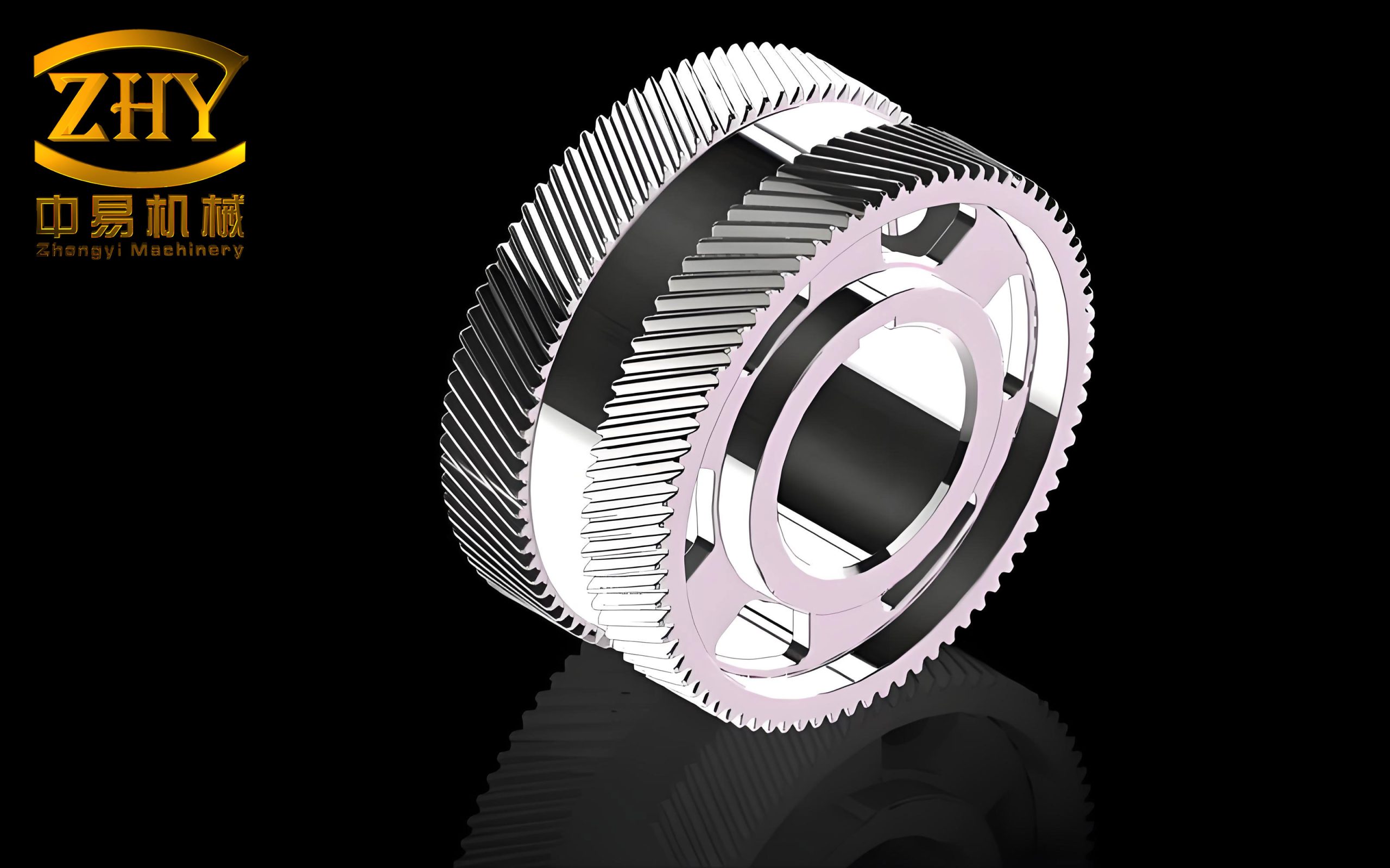
Dynamic Model of the Star Herringbone Gear System
I established a purely torsional lumped-parameter model for the star herringbone gear transmission. The model treats the sun gear, three planet gears, and the ring gear as rigid disks connected by nonlinear spring-damper elements along the line of action. Since the herringbone gear can be viewed as two opposite-handed helical gears assembled together, I modeled the left and right flanks separately. This approach accurately captures the helical angle effects and the mating phase differences among the planets. The equations of motion were derived using Newton’s second law.
For each gear body, the rotational displacement is denoted by θ with subscripts s for the sun, p for the planet, and r for the ring. The meshing between the sun gear and the i-th planet is represented by the relative displacement xspi, and that between the i-th planet and the ring by xrpi. The time-varying mesh stiffness k(t) is expressed as a Fourier series:
$$k_{spi}(t) = k_m \sum_{j=1}^{N} \varepsilon_j \sin\left(j \omega_m t + \varphi_{spi}\right) + k_m,$$
where km is the mean mesh stiffness, εj is the stiffness fluctuation coefficient, ωm is the meshing frequency, and φspi is the initial phase. Similarly, the mesh stiffness between the planet and ring gear is:
$$k_{rpi}(t) = k_m \sum_{j=1}^{N} \varepsilon_j \sin\left(j \omega_m t + \varphi_{rpi}\right) + k_m.$$
The mesh damping coefficient c is determined by the damping ratio ζ and the equivalent mass:
$$c = 2 \zeta \sqrt{k_m \frac{m_s m_p}{m_s + m_p}},$$
where ms and mp are the equivalent masses of the sun and planet gears, respectively. The damping ratio ζ is an important design parameter that directly influences the global dynamics.
To eliminate rigid-body displacements, I defined the relative displacements along the line of action:
$$x_{spi}^{(1)} = (r_s \theta_s^{(1)} – r_p \theta_{pi}^{(1)} – e_{spi}^{(1)}(t)) \cos\beta_1,$$
where rs and rp are the base circle radii, β is the helical angle, and e(t) is the composite transmission error, which is modeled as:
$$e_{spi}(t) = E \sin(\omega_m t + \varphi_{spi}^{(e)}).$$
A similar expression is used for the ring-planet meshing pair.
The gear backlash is a strong nonlinearity. The piecewise function g(u) is defined as:
$$g(u) =
\begin{cases}
u – b/2, & u > b/2,\\
0, & -b/2 \le u \le b/2,\\
u + b/2, & u < -b/2,
\end{cases}$$
where b is the dimensionless backlash, and u is the dimensionless relative displacement.
After introducing the dimensionless time τ = ωnt and the displacement scale L = 1×10⁻⁴ m, the dimensionless equations of motion can be written in matrix form as:
$$\mathbf{M} \ddot{\mathbf{U}} + \mathbf{C} \dot{\mathbf{U}} + \mathbf{K} \mathbf{g}(\mathbf{U}) = \mathbf{F},$$
where U is the vector of dimensionless relative displacements, M is the identity matrix (because the coordinates are the relative degrees of freedom), C and K are the dimensionless damping and stiffness matrices, and F is the dimensionless external load vector. The nonlinear function g(U) is applied elementwise according to the backlash piecewise law. This formulation ensures a well-posed system with a unique solution, as the mass matrix is positive definite and the stiffness matrix is symmetric positive definite.
The system parameters used in this study are summarized in Table 1.
| Parameter | Symbol | Value |
|---|---|---|
| Number of sun gear teeth | zs | 36 |
| Number of planet gear teeth | zp | 32 |
| Number of ring gear teeth | zr | 100 |
| Module | m | 4 mm |
| Pressure angle | α | 20° |
| Base helix angle | β | 22.5° |
| Sun gear mass | ms | 5.3018 kg |
| Planet gear mass | mp | 4.5099 kg |
| Ring gear mass | mr | 16.0843 kg |
| Sun gear inertia | Is | 0.0226 kg·m² |
| Planet inertia | Ip | 0.0149 kg·m² |
| Ring inertia | Ir | 0.6564 kg·m² |
| Mean mesh stiffness | km | 2×10⁹ N/m |
| Damping ratio | ζ | 0.1 |
| Backlash | b | 1×10⁻⁴ m |
Dynamic Response and Bifurcation Analysis
I solved the dimensionless differential equations using the fourth-order Runge–Kutta method with a fixed time step. The steady-state vibration was analyzed using phase diagrams, Poincaré sections, bifurcation diagrams, and the joint probability density of the attractor. The dynamic load coefficient was defined as:
$$K_v = \frac{k_m L g(u) + c \omega_n L \dot{u}}{F_{in}},$$
where Fin is the static load. A value close to unity indicates smooth meshing, while large fluctuations imply strong impact forces. The load-sharing coefficient was obtained by averaging the dynamic load coefficient over one meshing period.
Dynamic Load and Load-Sharing Characteristics
For the nominal operating condition of 9000 r/min and 3000 kW, the system exhibited intense vibrations, with the dynamic load coefficient varying between 0.2 and 2.8. By reducing the speed to 6000 r/min, the response became periodic with period 2, and the dynamic load coefficient for the sun-planet meshing pair approached unity, indicating a much smoother operation. The load-sharing characteristics were evaluated for different excitation parameters.
Table 2 summarizes the effects of the main excitation parameters on the load-sharing coefficient.
| Parameter variation | Trend of load-sharing coefficient | Observation |
|---|---|---|
| Increasing input power | Decreasing | Better load sharing at higher power |
| Increasing input speed | Increasing | Greater dynamic load at higher speed |
| Increasing damping ratio | Nearly constant | Minor influence |
| Increasing stiffness fluctuation | Slight decrease | Negligible effect |
| Increasing backlash | Increasing | More severe impact and instability |
Bifurcation Diagrams
I constructed bifurcation diagrams by plotting the Poincaré projection of the steady-state relative displacement usp1 against a gradually varying parameter. Figure 1 shows the bifurcation path as the sun-gear input speed n₁ increases from 4000 to 20000 r/min. The system repeatedly switches among period-1, period-2, period-4, quasi-periodic, and chaotic motions. Several jumping discontinuities are observed, indicating coexisting attractors and boundary crises.
For the input-power variation from 1500 kW to 4000 kW, the system evolves from chaotic motion to period-2 motion through a cascade of reverse period-doubling bifurcations. The response amplitudes decrease, and the vibration becomes more regular. A similar stabilizing effect was observed when the damping ratio was increased from 0.05 to 0.2. In contrast, increasing the stiffness fluctuation coefficient from 0.1 to 0.4 causes the system to lose stability and transition from period-4 to chaos. The backlash variation mainly affects the vibration amplitude; larger backlash leads to stronger impacts and higher amplitude, even though the periodicity may remain unchanged.
To validate the presence of the different attractors, I computed the joint probability density p(x,ẋ) over a long time series. For a period-1 attractor, the density function exhibits a single sharp peak; for period-2, two distinct peaks; and for chaotic attractors, a fractal, multi-humped distribution. These results confirmed the conclusions drawn from the bifurcation diagrams.
Experimental Verification
To ensure that the theoretical model was realistic, I built a star herringbone gear test rig. The test rig consisted of a variable-frequency motor, the herringbone gearbox, a magnetic powder brake, and two piezoelectric accelerometers placed on the bearing caps near the sun-planet meshing region. The motor speed was set to 1000, 1250, and 1500 r/min under a load of 2 N·m. The relative vibration acceleration was computed by subtracting the two accelerometer signals. Fast Fourier Transform (FFT) was used to obtain the frequency spectra. The measured first and second harmonics of the mesh frequency agreed well with the theoretical predictions, with small deviations attributed to manufacturing errors and bearing flexibility. This comparison validated the dynamic model and the subsequent numerical results.
Global Solution Domains and State-Space Attraction Basins
Local bifurcation analysis only reveals the response for one parameter while keeping others fixed. To gain a full picture of the star herringbone gear system, I employed the simple cell mapping method. The continuous parameter space or state space is discretized into a finite number of rectangular cells. Each cell is represented by its center point. Starting from the center, the system is integrated over one Poincaré period, and the image cell is determined. By repeatedly applying this mapping, the cell eventually falls into a periodic cell group or moves to a chaotic saddle. The period of the attractor can be identified by checking whether the image of a cell returns to itself after a certain number of steps.
For the parameter-domain analysis, I set the initial state to (0,0) and discretized the two-dimensional parameter plane into a 200×200 grid. The solution status of each parameter cell was classified as period-1 (P1), period-2 (P2), period-4 (P4), multi-period (Pn, n≥5), or chaos (Chaotic). The boundary cells were identified when the neighboring cells had different classifications. This procedure produced high-resolution parameter solution-domain maps that are difficult to obtain through one-dimensional sweeps.
Rotational Speed–Power Solution Domain
Figure 2 presents the parameter solution-domain map for the sun-gear speed n₁ in [3000, 20000] r/min and the input power P in [1500, 4000] kW. The dominant regions are P1, P2, P4, Pn, and chaotic zones. Along the speed axis, the periodic states change frequently, demonstrating the high sensitivity to rotational speed. Along the power axis, the system tends to approach P1 as the power increases, especially in the low-speed region. At high speeds, the system becomes more sensitive to power, and multiple periodicity changes occur. The map also reveals embedded islands of P4 inside the P2 region, indicating the coexistence of attractors and hysteresis.
I also extracted a vertical slice at n₁ = 11500 r/min and plotted the bifurcation diagram against power. The results matched the two-dimensional map: a transition from chaos to P4, then back to chaos, followed by P4, P2, and finally P4 again. This complex evolution shows that local bifurcation analysis alone cannot predict the effects of a second parameter.
Rotational Speed–Damping Ratio Solution Domain
Similarly, I computed the parameter solution-domain map for the speed-damping-ratio plane with Kem in [0.05, 0.2]. The map shows that a higher damping ratio generally stabilizes the system, driving it from chaotic or multi-periodic states to P1 or P2. However, at high speeds, the system can switch abruptly between P2, P3, P4, and P5 when the damping ratio changes slightly. Therefore, even though damping is beneficial, the operating point must be chosen carefully in high-speed conditions to avoid crossing an unstable boundary.
Power–Damping Ratio Solution Domain
The parameter map for power versus damping ratio covers P in [1500, 4000] kW and Kem in [0.05, 0.2]. At low power and low damping, chaotic cells dominate. As both parameters increase, the chaos region shrinks and is replaced by P2 and P4 regions. For Kem > 0.17, the system remains in P2 nearly independent of power. This map is useful for designers because it defines a safe operating zone.
State-Space Attraction Basins
The global attraction basin in the state space reveals which initial conditions converge to which attractor. I discretized the region u∈[−1,1] and u̇∈[−1,1] into 200×200 cells. For each cell, the system was integrated from the cell center, and the Poincaré points were recorded. The steady-state period was identified using the criteria:
$$|x_{k+\Delta}-x_k| < \varepsilon_1, \quad |\dot{x}_{k+\Delta}-\dot{x}_k| < \varepsilon_2, \quad \text{for } k=1,2,3,4,$$
where Δ is the number of discrete mapping steps and ε₁=ε₂=1×10⁻³. If no convergence was found after a maximum number of periods, the cell was classified as chaotic.
Figure 3 shows the evolution of the state-space attraction basins for increasing input power at n₁=9000 r/min. At P=2800 kW, the basin consists of 21% P2 cells, 1% P4 cells, 60% chaotic cells, and the rest multi-periodic cells. The boundaries between basins are highly interwoven, meaning that small perturbations in the initial state can drastically change the final response. At P=3000 kW, the chaotic portion decreases to 7%, and P2 grows to 23%. At P=3200 kW, the chaotic cells disappear entirely; the system is partitioned into a 34% P2 basin and a 30% P4 basin, with the remaining multi-periodic cells. This shows that increasing power suppresses chaos and reduces the sensitivity to initial conditions.
I also studied the effect of the damping ratio. At Kem=0.08, 85% of the state space is chaotic. At Kem=0.10, the chaotic fraction drops dramatically, and at Kem=0.12, the entire basin is composed solely of P2 and P4 attractors: 35% P2 and 65% P4. Thus, increasing the damping ratio is an effective way to simplify the global basin structure and improve stability.
Random Excitation and Global Dynamics
In real machinery, the excitation parameters are never exactly constant. They fluctuate randomly due to manufacturing tolerances, load variations, speed ripples, and thermal effects. To model these uncertainties, I generated normally distributed pseudo-random numbers using the central limit theorem and the limit approximation method:
$$\eta = \mu + \sigma \cdot \frac{\sum_{i=1}^{12} U_i – 6}{\sqrt{1}},$$
where Ui are independent uniform random variables in (0,1), μ is the mean value of the excitation parameter, and σ is the standard deviation. The random number was accepted only if it fell within the specified upper and lower limits; otherwise, it was regenerated. This approach preserves the mean and variance of the original parameter while imposing physically realistic bounds.
I applied the random excitation separately to the damping ratio, input power, input speed, and backlash, and then recomputed the state-space attraction basins. Table 3 summarizes the qualitative changes in the global dynamics compared with the deterministic case.
| Random parameter | Distribution | Effect on global basin |
|---|---|---|
| Damping ratio ζ | N(0.1, 0.0002²) | Small deterioration: basin boundaries become blurred; a few chaotic cells appear; P2 and P4 fractions slightly decrease. |
| Input power P | N(3200, 3²) | Minimal change: P2 and P4 fractions slightly increase; multi-periodic cells shrink; beneficial effect. |
| Input speed n₁ | N(9000, 3²) | Severe deterioration: 63% of the basin becomes chaotic; P2 and P4 basins are completely destroyed; the system is extremely sensitive to speed fluctuations. |
| Backlash b | N(1, 0.002²) | Very severe: 69% chaotic cells; the remaining periodic cells are scattered; initial-condition sensitivity becomes extreme. |
Figure 4 shows a typical attraction basin when the damping ratio contains a random fluctuation of variance 0.0002². The basin structure is globally similar to the deterministic case, but the boundaries are more irregular, and some state cells switch their attractor classification. When the variance increases to 0.0004², the P2 basin largely transforms into P4, and the chaotic fraction grows to about 2%. The dynamic response of a selected cell changes from a clean period-2 oscillation to a quasi-periodic oscillation with drifting amplitude, demonstrating that random damping worsens the vibration regularity.
In contrast, random fluctuations in the input power have a slightly favorable effect. The fractions of P2 and P4 attractors increase, and some multi-periodic cells convert to period-2 cells. This result suggests that minor power fluctuations can sometimes help the system escape from a weakly stable multi-periodic state. However, this improvement is accompanied by a higher sensitivity to initial conditions because the basin boundaries become more distorted.
The worst effects are caused by random input speed and random backlash. Since the deterministic system at n₁=9000 r/min lies close to a boundary between periodic and chaotic domains, even a tiny speed fluctuation pushes many cells into chaos. The global basin becomes a mosaic of chaotic and multi-periodic regions with no clear domain structure. The same happens when the backlash fluctuates randomly around b=1. The strong nonlinearity of backlash amplifies the random perturbation, leading to a 69% chaotic occupancy. These findings highlight the importance of precisely controlling speed and backlash in high-performance herringbone gear transmissions.
From the random excitation analysis, I derived practical recommendations:
- Select operating points inside a stable P1 or P2 region in the parameter solution-domain map to avoid chaotic boundaries.
- Increase damping ratio and input power moderately to reduce the negative impact of random fluctuations.
- Improve manufacturing precision and mount design to minimize backlash randomness and speed ripples.
- Acceptable tolerance for input power variation is larger than for speed or backlash variations.
Conclusions
This research investigated the global dynamics of a star herringbone gear transmission system through a combination of nonlinear numerical analysis, cell mapping, and random excitation simulation. The main conclusions are:
1. The pure torsional dynamic model with time-varying mesh stiffness, backlash, and transmission error is effective for predicting dynamic loads and stability trends. The fourth-order Runge–Kutta solution and experimental validation confirmed the accuracy of the model.
2. The star herringbone gear system exhibits rich bifurcation behavior. Increasing speed tends to promote chaos and period-doubling cascades, while increasing power and damping ratio stabilize the system. Stiffness fluctuation always reduces stability, and backlash mainly increases vibration amplitude.
3. The two-dimensional parameter solution-domain maps provide a comprehensive view of the system’s periodic and chaotic regions. These maps reveal coupling effects between parameters, including embedded islands of higher-period attractors inside lower-period regions, which are invisible in one-dimensional bifurcation plots.
4. State-space attraction basins show that the system’s global stability strongly depends on initial conditions. At low power or low damping, chaotic basins dominate and the system is highly sensitive to initial-state perturbations. As power or damping increases, the basins become simpler and consist mainly of period-2 and period-4 attractors, which improves the system’s overall robustness.
5. Random excitations generally deteriorate the global dynamic behavior. The deterioration increases with the variance of the random fluctuation. Input speed and backlash are the most critical random parameters; they can cause a sudden transition to global chaos even when the deterministic system is stable. Input power is the least critical parameter, and its small random variation may even improve the basin structure.
6. The combination of cell mapping, parameter solution domains, and random excitation simulation provides a powerful framework for the global design and optimization of star herringbone gear transmission systems. By selecting safe parameter zones and minimizing random fluctuations of sensitive parameters, engineers can effectively mitigate nonlinear vibrations, avoid chaos, and enhance the reliability of herringbone gear drives.
Future work should extend the present model to include tooth friction, dynamic wear, and multi-body effects. The cell mapping method can also be coupled with intelligent optimization algorithms to automatically search for the most stable parameter combination. The proposed global analysis procedure is not limited to herringbone gears; it can be applied to any nonlinear gear system with multiple excitation sources.