
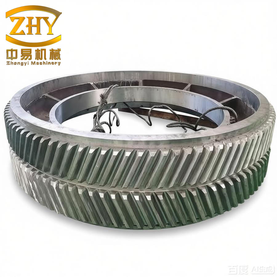
Herringbone gears consist of two helical gears with the same helix angle but opposite hand directions, which are arranged side by side. They possess the advantages of excellent load-carrying capacity and stable transmission without impact, inherited from helical gears, while their unique configuration effectively cancels axial forces generated during meshing. Consequently, herringbone gears are widely applied in heavy-duty machinery transmissions.
In my research, I investigated the machining of recess-free herringbone gears. Traditional manufacturing processes for herringbone gears typically involve hobbing for rough machining followed by grinding for finishing. However, these conventional approaches necessitate designing a recess (also known as a “withdrawal groove” or “gill” in some contexts) at the gear’s center to prevent tool interference. I identified that this recess increases the gear’s axial dimensions, compromises gearbox compactness, and diminishes gear teeth alignment between the left-hand and right-hand sections. To eliminate the need for this recess, I employed end mills for flank milling on multi-axis CNC machining centers. This method achieves superior gear teeth centering and bending strength at the tooth root, and importantly, avoids the costs and lead times associated with custom-designed dedicated tools. My approach demonstrated significant advantages in manufacturing small batches of herringbone gears with varying module, teeth numbers, and pressure angles when compared to conventional processing.
1. Introduction and Research Background
Gear transmission systems are among the most extensively used power transmission mechanisms in the mechanical industry, with applications spanning wind power, automotive, marine, aviation, and instrumentation sectors. Through my analysis, I recognized that herringbone gear transmission is an essential component within these systems. Environmental considerations and performance demands driven by modern applications require continuous process improvements. Traditional manufacturing, while effective in mass production scenarios, possesses specific limitations that become pronounced in certain niche applications.
The standard industry practice for fabricating herringbone gears involves utilizing a hob cutter for the roughing stage and a grinding wheel for final finishing. During such processing, a pre-machined groove at the gear’s center becomes mandatory to prevent interference between the tool and the workpiece. However, this groove, termed a “relief groove” or “recess,” introduces several undesirable effects. It increases the gear’s axial dimension and weight, reduces gearbox compactness, and, perhaps most critically, creates poor alignment (poor centering) between the left-hand and right-hand teeth. Additionally, hobbing cutters and grinding wheels are specialized, application-specific tools. Developing these tools typically requires a lead time of one to two months, and the overall costs can be substantial since each cutter is designed for a specific module and pressure angle.
My research addresses these limitations by utilizing general-purpose end mills on programmable CNC machining centers. Unlike disc-shaped hobs or grinding wheels, end mills have a cylindrical form whose diameter is smaller than the gear tooth slot dimensions. This geometry permits flank milling operations without interference, thereby eliminating the need for the recess. I confirmed that this approach results in favorable gear tooth alignment and improved bending strength. The advantage becomes particularly evident in low-volume production runs involving different gears of different module, tooth count, or pressure angle specifications, where the custom tool costs of hobbing or grinding are prohibitive and the lead times are unacceptable. Three primary non-traditional methods for machining recess-free herringbone gears are described in the literature: gear shaping with two cutters, gear planing with comb cutters, and gear milling with finger cutters. However, these methods have inherent drawbacks, such as expensive, difficult-to-manufacture tooling, limitations on module size, or lower achievable precision. My work focuses on a superior alternative.
2. Machining Program for Recess-Free Herringbone Gears
2.1 Three-Dimensional Solid Modeling
For my study, I utilized the example of a recess-free herringbone gear with the design parameters specified in Table 1, based on a design document. The solid model was established using Siemens NX 10.0 software. I employed two approaches: constructing the standard involute and helical geometry via formula-driven curves, and utilizing the “GC Toolbox” module which allows rapid creation of gears meeting Chinese GB standards. It is worth noting that the GC Toolbox is accessible only in the Chinese language environment of the software. Using the latter, I input the parameters from Table 1, creating the 3D model efficiently. The process involved creating a helical gear and subsequently using the “Mirror Geometry” command to generate the complete herringbone gear from the helical gear.
| Module m (mm) | Number of teeth z | Addendum coefficient han* | Pressure angle α (°) | Helix angle β (°) | Clearance coefficient c* |
|---|---|---|---|---|---|
| 16 | 30 | 1.0 | 20 | 30 / -30 | 0.25 |
2.2 Tool Selection and Machining Methodology
The selection of cutting tools is crucial for achieving the desired precision and process efficiency. In machining curved surfaces on CNC machines, ball-end mills and flat-end mills (end mills) are commonly used. My analysis showed that while ball-end mills are versatile for free-form surfaces due to their constant radius geometry, which simplifies tool center positioning, they suffer from low cutting speed and poor chip evacuation near their rotational center. In contrast, for machining convex surfaces like involute gear teeth flanks, which have relatively minor curvature variations, flat end mills are advantageous as they yield a larger machining strip width, larger stepover distances, and therefore, lower machining time. Considering the gear surface, which is an involute helicoid from the flank milling perspective, I selected flank milling with a flat end mill for the semi-finishing and finishing operations of the tooth flanks. A ball-end mill was chosen for machining the tooth root fillet.
Regarding the milling strategy, I decided to use down-milling (climb milling) over up-milling (conventional milling) because climb milling provides a better surface finish, reduces tool wear, and prevents the workpiece from being lifted off the fixture. This is especially important for achieving the high surface quality required for gear flanks.
Given that the gear requires carburization to achieve a surface hardness of HRC 58–62 and a core hardness of HRC 30–40, the material is categorized as hard steel. Based on this, I selected PVD-coated solid carbide end mills, which offer superior wear resistance, high heat resistance, and higher permissible cutting speeds than high-speed steel tools. To determine appropriate tool sizes, I measured the tooth slot geometry of the solid model. I determined that the tooth slot bottom has a minimum internal clearance of 7.5373 mm, and the distance between the tooth root fillets’ tops is 16.625 mm. Consequently, I selected the following tools:
- ϕ20 mm solid carbide end mill for the roughing of the tooth slot except the bottom region (interference-free area).
- ϕ10 mm solid carbide end mill for roughing of the tooth slot bottom.
- ϕ12 mm solid carbide end mill for semi-finishing and finishing of the tooth flanks.
- ϕ8 mm solid carbide ball-end mill for semi-finishing and finishing of the tooth root fillet.
I determined the tool geometry parameters: helix angle of 40° for the ϕ20 mm mill and 30° for the ϕ12 mm mill. I selected a rake angle of 10° for steel machining and a clearance angle of 12° for the ϕ20 mm mill and 15° for the ϕ12 mm mill. The cutting parameters, established based on the tool manufacturer’s recommendations and standard machining tables, are compiled in Table 2.
| Process Stage | Programming Method | Tool Type / mm | Spindle Speed / (r/min) | Feed Rate / (mm/min) |
|---|---|---|---|---|
| Rough opening of tooth slot | Variable axis contour milling | ϕ20 flat-end mill | 800–1200 | 500 |
| Rough milling slot bottom | Variable axis contour milling | ϕ10 flat-end mill | 800–1200 | 500 |
| Semi-finish milling flank | Variable axis contour milling | ϕ12 flat-end mill | 2300–3000 | 500 |
| Semi-finish milling slot bottom | Variable axis contour milling | ϕ10 flat-end mill | 2300–3000 | 500 |
| Semi-finish root fillet | Variable axis contour milling | ϕ8 ball-end mill | 2500 | 500 |
| Finish milling flank | Variable axis contour milling | ϕ12 flat-end mill | 2500 | 500 |
2.3 NC Program Generation using UG CAM
I used the NX CAM module to generate the toolpaths for the herringbone gear processing. The workflow involved creating a program order, setting up the machining coordinate system, defining the stock (a cylinder with a diameter equal to the outside diameter of the gear and height equal to the face width), and defining the safe plane. I utilized the “Variable Contour” operation within the multi-axis milling environment to generate all necessary toolpaths. The basic settings included establishing the coordinate system origin at the center of the gear’s reference circle and fixture offset.
To create the rough machining operation, I generated a toolpath using the “Surface Area” driving method. In this case, an auxiliary plane was created in the middle of the tooth slot, and this plane was selected as the drive geometry. The projection vector was set to “Tool Axis”, and the tool axis was set to “4-Axis Relative to Drive”. A “Zig-Zag” cut pattern was selected, and the toolpath was generated. To machine the tooth slot bottom region with the ϕ10 mm end mill, I copied this operation, selected the same driving surface, and adjusted the “Start Step” and “End Step” percentages (from 60% to 95%) in the surface driving method dialog box to limit the area covered by the toolpath. This strategy reduced the cutting depth to avoid the risk of over-cutting with the larger ϕ20 mm mill in the restricted space near the bottom of the slot.
For semi-finishing of the flanks, a similar “Variable Contour” operation was created using the same driving method and milling mode, but with the gear flank selected as the drive surface. To leave stock for the finishing operation, I set the “Offset” parameter to 1 mm. The finishing operation for the tooth flank utilized the “Zig” (one-way) cut pattern to maintain the specified down-milling strategy and set the “Offset” to 0. I noted that the use of a one-way cutting pattern is critical here for achieving the required surface finish and precision. The root fillet and tooth slot bottom finishing operations were programmed using the ϕ8 mm ball-end mill with a similar “Variable Contour” approach.
The 3D dynamic simulation capability within UG NX CAM was used to perform a preliminary inspection, verifying that the generated toolpaths were free from any gross interference or over-cutting. The roughing toolpaths, flank finishing toolpaths, and root fillet finishing toolpaths were visually inspected and adjusted if needed.
3. Optimization of Flank Finishing Toolpaths Using Constant Scallop-Height Method
3.1 Theoretical Foundation
The tooth flank of a helical gear is an involute helicoid. For an involute curve in a planar coordinate system, the profile can be described with the following parametric equations:
In Cartesian coordinates, the involute can be expressed as:
$$ \begin{cases} x = r_b (\cos\varphi + \varphi \sin\varphi) \\ y = r_b (\sin\varphi – \varphi \cos\varphi) \end{cases} $$
where:
- \( r_b \) is the radius of the base circle;
- \( \varphi = \alpha + \theta \) is the roll angle, where \( \alpha \) is the pressure angle and \( \theta \) is the polar angle.
To define the helicoid of a helical gear tooth flank, the involute curve is subjected to a helical motion around the gear axis. Let \( h \) be the lead of the helix, and \( \mu \) be the helical motion parameter. The general equation of the involute helicoid is obtained by combining the involute equations with the helical transformation:
$$ \begin{cases} x = r_b [\cos(\varphi + \mu) + \varphi \sin(\varphi + \mu)] \\ y = r_b [\sin(\varphi + \mu) – \varphi \cos(\varphi + \mu)] \\ z = \dfrac{h}{2\pi} \mu \end{cases} $$
Here, \( \mu \) represents the parameter for the helical motion. For a constant \( \mu \), the equations represent different involute profiles. Conversely, for a constant \( \varphi \) (a point on the base circle), varying \( \mu \) traces a helix. At a given radius \( r \), the helix angle \( \beta_r \) can be calculated using:
$$ \tan\beta_r = \dfrac{2\pi r}{h} $$
My key task is to optimize the toolpath for flank finishing. I established that the use of the traditional iso-parametric method is inefficient for finishing the involute helicoidal flank. This is because the curvature radius of the involute profile varies significantly from its starting point at the base circle to its endpoint at the outside diameter of the gear. The minimum curvature radius occurs at the involute’s starting point. The iso-parametric method obliges the programmer to select a stepover distance based on the smallest curvature radius to ensure the scallop height does not exceed the tolerance in that region. This results in an excessive number of toolpaths across the rest of the flank, and a huge waste of machining time.
To address this issue, I adopted the Constant Scallop-Height method. The principle of this method is to maintain the maximum scallop height (residual height) constant across the entire surface while ensuring it does not exceed the specified tolerance. This allows the stepover distance to be maximized locally, especially in areas with larger curvature radii, thereby reducing the total number of toolpaths. The relationship between the curvature radius \( r \), scallop height \( \lambda \), and stepover distance \( l \) (Figure 3-1 from my original work) is derived from geometry as:
$$ l \approx \sqrt{\dfrac{8\lambda r}{1 \pm \dfrac{r}{R}}} $$
In this equation, \( R \) is the tool radius. For a flat end mill in flank milling, the effective cutter radius might be considered as a modified value depending on the context of contact. For simplicity, and when the work curvature radius is significantly larger than the tool radius, the approximation:
$$ l \approx \sqrt{8\lambda r} $$
is often applied. A positive sign is used for concave surfaces and a negative sign for convex surfaces. This formula confirms that the stepover distance \( l \) increases with an increasing curvature radius \( r \), when the scallop height \( \lambda \) is constant.
3.2 Numerical Analysis and Verification
I used Matlab software to analyse the relationship between these variables for the specific gear in my research. The curvature radius at the involute starting circle is \( r_{min} = 77.366 \) mm, and at the outside diameter is \( r_{max} = 143.821 \) mm. To meet the ISO 6 precision grade requirement for the gear, I set the maximum scallop height \( \lambda = 0.0025 \) mm. The Matlab analysis shows the calculated stepover distances from the start of the involute to the outside diameter vary from 1.2 mm to 1.7 mm, confirming that a significant amount of toolpath redundancy would result from using a single, constant, minimum stepover across the entire flank.
My method for planning the flank finishing toolpaths for herringbone gears based on the constant scallop height is described here. I use the flank profile for the calculation. Let \( g(x) \) be the involute curve. To find the next cutting point \( C(x_c, y_c) \) given a current point \( A(x_0, y_0) \), I first generate an offset curve \( f(x) \) that is at a distance of \( \lambda \) (the residual height) from \( g(x) \) along its normal direction, pointing away from the base circle:
$$ f(x, y) = g(x, y) + \lambda \cdot \vec{n}(x, y) $$
Then, I generate a tangent line to the involute at point A. The line has the equation:
$$ L_A: y – y_0 = g'(x_0)(x – x_0) $$
I find the intersection point \( B(x_b, y_b) \) between this tangent line \( L_A \) and the offset curve \( f(x) \). The point \( B \) is the tangent point of the next toolpath’s tangent line. Next, I construct a tangent line to the involute \( g(x) \) at a candidate point \( C(x_c, y_c) \). I find the point \( C \) such that the tangent line at \( C \) passes through \( B \). The slope condition is:
$$ g'(x_c) = \dfrac{y_b – y_c}{x_b – x_c} $$
Solving this equation yields the coordinates of the next tool contact point \( C \). Point A and point C are the adjacent cutting points that ensure the scallop height is equal to \( \lambda \). I repeated this process recursively until the entire involute profile, from the outside diameter to the involute starting circle, is covered.
In my example of the 30-tooth herringbone gear, I made the following observations. The constant scallop-height method generated 21 toolpath contact lines across the flank profile. The iso-parametric method, using the minimal stepover and the largest number of toolpaths needed to satisfy the tolerance condition, required 25 toolpath contact lines. The constant scallop-height method thus generated 4 fewer toolpaths, a 16% reduction in the number of passes across a single flank. In the machining of a complete herringbone gear (30 teeth), this amounts to a reduction of 120 flank passes (30 teeth × 2 flanks × 4 paths less). The calculated stepover values obtained from the constant scallop-height method are shown in Table 3.
| Stepover Number | Stepover Value (mm) | Stepover Number | Stepover Value (mm) |
|---|---|---|---|
| 1 | 1.6864 | 11 | 1.4855 |
| 3 | 1.6499 | 14 | 1.4094 |
| 6 | 1.5908 | 18 | 1.2989 |
| 10 | 1.5063 | 20 | 1.2346 |
To generate the tool center path from the tool contact path, I offset each point on the contact line by a value equal to the tool radius \( R_{tool} \) along the normal vector of the involute flank. The resulting tool path is a line that follows the helix at its specific radius. In the flank milling context, this is effectively an offset of the tool contact path in the direction normal to the machined surface.
If \( t \) is the time to machine one toolpath, the time saved \( T \) when machining a complete herringbone gear is calculated as:
$$ T = 4 \cdot t \cdot z $$
where \( z \) is the number of teeth (z=30). This provides a direct measure of the efficiency gain.
4. Development of a Toolpath Generation Program Using UG Secondary Development
The constant scallop-height toolpath generation is complex and repetitive. To improve programming efficiency and reduce potential errors, I developed a secondary development program within Siemens NX. I chose the Knowledge Fusion (KF) language for this purpose, as it is a powerful, rule-based design language integrated within NX, enabling the creation of custom features and automated design tasks. Before starting the development, I created a folder structure within the NX installation directory, with “startup” and “application” subfolders, and set the proper environment variable to allow NX to access my customizations.
First, I designed a custom menu in a “*.men” file placed in the “startup” folder. The menu, labeled “无槽人字齿轮等残高精加工” in my original work, is displayed in the main NX menu bar. The menu calls the custom KF program using an ACTIONS command. I also developed a custom UI interface using the UI Editor (UIStyler). This interface was designed to be user-friendly, allowing the user to:
- Select the pre-defined set of points (the computed constant scallop-height contact points).
- Input the required helical gear parameters: base circle radius \( r_b \), helix angle \( \beta \), lead \( h \), and the data point radius \( r_x \).
- Visualize a schematic representation of the machining program to understand the function’s intent.
I used the “point-line method” or “point method” for the secondary development. The process consisted of two main steps:
- Calculation of contact points using MATLAB: I wrote a MATLAB script to calculate the constant scallop-height cutting points (刀触点). Starting from the known intersection of the outside diameter and the involute curve \( A(x_0, y_0) \), I used an iterative search algorithm based on the tangent-offset curve method to compute subsequent points \( B \), \( C \), etc., until reaching the involute starting circle (the condition \( x_{n+m}^2 + y_{n+m}^2 \le r_0^2 \) where \( r_0 \) is the starting circle radius). These points were saved and imported into NX as point geometry objects.
- Development of the Helix Generation Program in KF: I used the KF language to create a custom class that iterates through the selected points. For each point, the program calculates the local helix angle based on the point’s radial distance \( r \) and the user-defined lead \( h \):
$$ \beta_r = \arctan\left(\dfrac{2\pi r}{h}\right) $$
Using the “ug_spline_thru” command within a “for” loop, I generated a spline (the helix) through the predetermined points at that radial distance. By connecting these splines, the complete set of flank milling toolpaths based on the constant scallop-height principle is generated.
The choice of the point method over the modeling method (which uses offset and intersection commands directly in the NX model) was deliberate. The modeling method, while conceptually simpler, only creates the toolpath on the geometric model, and is less flexible. My point-line method, however, generates true 3D spline curves that can be post-processed into machine code, and is more robust for the varying helix angles found in helical gears. This program greatly simplified the task of generating the optimized toolpaths, as it integrated the MATLAB calculation with the NX environment using a custom user interface.
5. Simulation and Experimental Verification
5.1 VERICUT Simulation Setup
Prior to physical cutting trials, I utilized VERICUT software to simulate the entire machining process. This was crucial for verifying the NC program’s correctness, detecting potential collisions or over-cuts, and estimating the machining cycle times. I modeled the DMU 210FD mill-turn machining center, including its kinematic chain, travels, and controls. I then created the cutting tools in VERICUT’s tool manager:
- ϕ20 flat end mill: Diameter (D) = 20 mm, Length (H) = 92 mm, Cutting edge length = 26 mm
- ϕ12 flat end mill: Diameter (D) = 12 mm, Length (H) = 83 mm, Cutting edge length = 26 mm
- ϕ8 ball end mill: Diameter (D) = 8 mm, Length (H) = 100 mm, Cutting edge length = 16 mm
Standard tool holders for these tools were modeled using basic 3D shapes (cylinders and a cone). The tool holder coordinates were set correctly to assemble the tools and holders. A simplified but dimensionally accurate fixture was modeled as a ϕ480 mm × 450 mm cylinder. The final setup is shown in the VERICUT environment.
The machine model was selected as the DMU 210FD. The NC program, generated by the post-processor from the UG CAM toolpaths, was loaded. The coordinate system was aligned, and the simulation was executed. The simulation confirmed that the programs were error-free in terms of gouging and collisions. The simulation also recorded processing times.
The VERICUT simulations showed that the iso-parametric method took 24 minutes and 22 seconds to machine a single tooth flank, whereas the constant scallop-height method took only 19 minutes and 4 seconds. These results are presented in Table 4.
| Method | Machining Time for One Flank |
|---|---|
| Iso-parametric method | 24 min 22 sec |
| Constant scallop-height method | 19 min 4 sec |
5.2 Experimental Machining and Measurement
I performed the actual machining experiments on a DMU 210FD machining center. The gear blank, made of 45 carbon steel, was mounted on a custom-designed fixture. To prevent the workpiece from rotating during machining, I designed a key connection between the fixture’s end face and the gear blank’s end face. A standard flat key with dimensions of 10 mm × 36 mm × 8 mm was used to restrict the rotational degree of freedom. The gear blank was clamped securely using a pressure plate and bolts. After setup, a probe was used to locate the workpiece’s center of rotation and ensure that the radial and axial runout values were less than 0.01 mm.
Following the process plan, the gear was machined. The machining used cutting fluid to cool and lubricate the cutting zone. During the operations, I monitored the machining noise and adjusted the feed and speed override as necessary. After roughing, I inspected the tool wear. For finishing tests, I used both NC programs: one with the iso-parametric toolpaths and the other with the constant scallop-height toolpaths, applying each to machining the flank surfaces. I measured the actual machining time for each flank finishing pass. The results are summarized in Table 5.
| Method | Simulated Time per Tooth (min) | Actual Time per Tooth (min) |
|---|---|---|
| Iso-parametric method | 48.73 | 63.0 |
| Constant scallop-height method | 38.00 | 51.2 |
The actual machining times are longer than the simulated times, mainly due to the time spent for operator checks, tool changes, and manual adjustments during the test. Nevertheless, the relative efficiency improvement is clear. The constant scallop-height method reduced the actual per-tooth machining time from 63 minutes to 51.2 minutes. For the entire gear, this results in a total saving of 5 hours and 54 minutes (approximately 19% reduction) compared to the iso-parametric method. The total estimated machining time for the complete gear using my CNC process was around 80 hours, including roughing, semi-finishing, and finishing.
After machining, I measured the gear using a Gleason 1500GMS gear measuring machine. The measurement process involved:
- Setting up the gear workpiece on the machine’s table.
- Inputting the gear parameters (module, pressure angle, etc.) to create a virtual master gear.
- Using a probe to align the gear’s rotational center with that of the measuring machine.
- Establishing the measurement coordinate system and running the measurement program.
The measurement report is included in my thesis appendix. The key measurement results are summarized in Table 6.
| Parameter | Max Value (μm) | Min Value (μm) | Average Value (μm) | GB Grade 6 Tolerance (μm) |
|---|---|---|---|---|
| Total profile deviation \( F_\alpha \) | 11.3 | 7.6 | 9.7 | 23 |
| Profile form deviation \( f_{f\alpha} \) | 9.2 | 3.8 | 5.8 | 18 |
| Profile slope deviation \( f_{H\alpha} \) | 10.0 | 5.7 | 7.6 | ±15 |
| Total helix deviation \( F_\beta \) | 11.5 | 10.3 | 10.8 | 18 |
| Helix form deviation \( f_{f\beta} \) | 3.3 | 2.6 | 3.0 | 13 |
| Helix slope deviation \( f_{H\beta} \) | 11.7 | 10.5 | 11.1 | ±13 |
5.3 Analysis of Measurement Results
The measurement results confirm that the machined recess-free herringbone gears meet the required ISO 6 (GB) precision grade. All six measured parameters — total profile deviation, profile form deviation, profile slope deviation, total helix deviation, helix form deviation, and helix slope deviation — are well within the specified tolerances. The profile total deviation reached a maximum of 11.3 μm, the helix total deviation a maximum of 11.5 μm, and the helix angle deviation a maximum of 0.0054°. This validates that the constant scallop-height method, when applied in this manner, is a viable and effective strategy for producing precision herringbone gears.
Upon analysis of the measurement reports, I observed consistent helix deviations. I identified three potential causes for this phenomenon:
- Modeling accuracy: The helical gear model may have slight inaccuracies in the helix geometry generated in the CAM software, which are transferred to the toolpaths.
- Cutting tool wear: Progressive flank wear on the cutting edges of the end mills during long machining operations can introduce dimensional or geometric deviations.
- Setup and stability: Minor movement or deflection in the workpiece setup, particularly in the key connection and clamping system, and any low-frequency vibration (chatter) during the cutting process, can contribute to the observed pattern.
I proposed several corrective actions to mitigate these effects: increase the precision of the helix geometry in the CAD model, implement a more rigorous tool wear monitoring and change-out schedule, and fine-tune the cutting parameters (spindle speed and feed rate) to minimize machining vibrations.
6. Conclusion and Future Outlook
In my thesis, I successfully demonstrated the complete methodology for machining recess-free herringbone gears on multi-axis CNC machines using off-the-shelf end mills. The following summarizes the contributions and findings of my research:
- Process development: I developed a complete and practical machining plan for recess-free herringbone gears, including tool selection based on gear geometry, cutting parameter selection based on workpiece material, and process sequencing.
- Toolpath optimization: I adapted the constant scallop-height principle to the specific challenge of gear flank milling. My method significantly reduces toolpath length and machining time by rationally distributing the stepover across the involute profile.
- Software development: I significantly improved programming efficiency by creating a dedicated software program that automates the generation of constant scallop-height toolpaths. The integration of MATLAB for contact point calculation and NX Knowledge Fusion for toolpath generation provides a streamlined, user-friendly workflow.
- Verification and validation: The effectiveness of the proposed methodologies was confirmed via VERICUT simulations and actual machining trials on a DMU 210FD machine. The machined gear exceeded the design requirements, achieving a GB 6 precision grade.
- Efficiency gains: My work confirmed that the constant scallop-height method is significantly more efficient than the iso-parametric method for machining herringbone gears, achieving a 19% reduction in total machining time for the test case. This translates into substantial cost savings and productivity improvements in a production environment.
Several opportunities for improvement and future research have been identified:
- Tool axis vector optimization: In the machining of the tooth root fillet with a ball-end mill, the analysis showed a need to optimize tool axis vector to avoid cutting near the center of the ball-end mill where the cutting speed approaches zero, which is detrimental to surface integrity and tool life.
- Bi-directional milling strategy: While my finishing strategy used a one-way (conventional) down-milling approach to achieve the required surface finish, the possibility of using a zig-zag or bi-directional strategy should be explored to further reduce machining time, although its impact on the achievable precision and surface quality would need to be thoroughly investigated.
- Extension to profile-modified gears: my current methodology is specifically for standard involute gears. Future work should focus on adapting the constant scallop-height toolpath generation method to accommodate gears with profile or lead modifications (e.g., tip relief, root relief, or crowning), which are essential for many heavy-duty applications.
In conclusion, this research provides a valuable new solution for the manufacturing of recess-free herringbone gears and opens up new avenues for the design of next-generation, more compact, and higher-performing herringbone gearboxes.