
I have focused my work on the dynamic characteristics and modification optimization of high-speed train helical gears under multiple operating conditions. In high-speed train transmission systems, helical gears are critical components because they directly influence running stability, safety, reliability, vibration, and acoustic behavior. I treat the helical gears as a coupled mechanical system in which time-varying mesh stiffness, friction, backlash, static transmission error, and dynamic transmission error interact. My objective is not to optimize helical gears for one fixed working point but to obtain a set of modification parameters that can improve the overall dynamic behavior of helical gears across nine representative operating conditions.
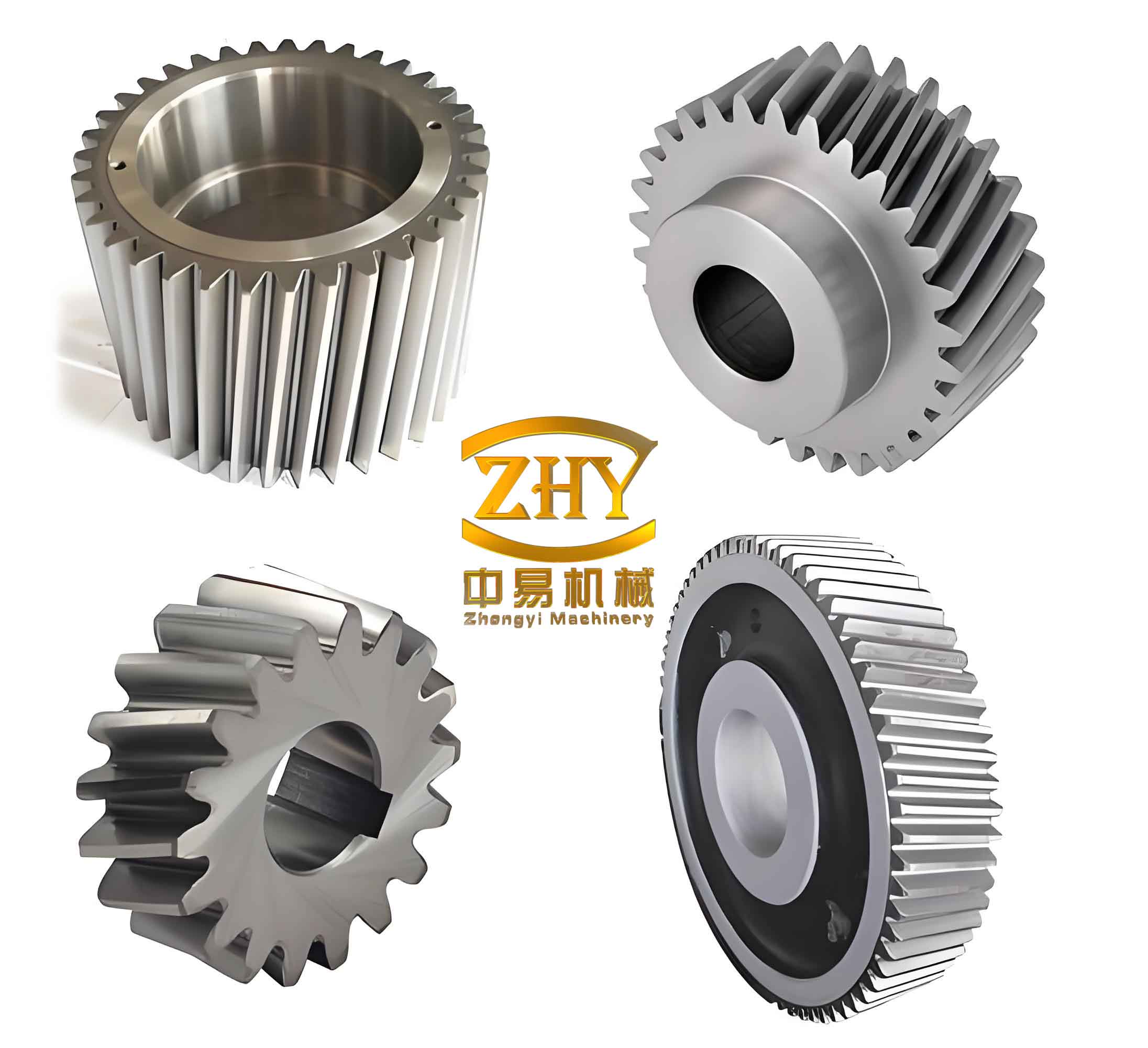
I begin with a lumped-parameter dynamic model of helical gears. The model is a six-degree-of-freedom translational-bending-torsional system. I use generalized coordinates for the driver and driven helical gears, including two lateral displacements and one angular displacement for each gear. The coordinate vector is written as
$$
\mathbf{q}=[x_1,\;x_2,\;y_1,\;y_2,\;\theta_1,\;\theta_2]^T .
$$
For helical gears, the line of action is not purely in one lateral direction because the helix angle couples axial, lateral, and torsional behavior. I simplify the model by projecting the normal mesh force and friction force into the lateral directions and by retaining the torsional degrees of freedom. The equations of motion can be summarized as
$$
\begin{aligned}
m_1\ddot{x}_1+c_{x1}\dot{x}_1+k_{x1}x_1&=-F_n\cos\beta-F_f\sin\beta,\\
m_2\ddot{x}_2+c_{x2}\dot{x}_2+k_{x2}x_2&=F_n\cos\beta+F_f\sin\beta,\\
m_1\ddot{y}_1+c_{y1}\dot{y}_1+k_{y1}y_1&=F_f\cos\beta-F_n\sin\beta,\\
m_2\ddot{y}_2+c_{y2}\dot{y}_2+k_{y2}y_2&=-F_f\cos\beta+F_n\sin\beta,\\
I_1\ddot{\theta}_1&=T_1-F_n r_{b1}+T_{f1},\\
I_2\ddot{\theta}_2&=-T_2+F_n r_{b2}-T_{f2}.
\end{aligned}
$$
Here, \(m_1\) and \(m_2\) are the masses of the driver and driven helical gears, \(I_1\) and \(I_2\) are their rotary inertias, \(r_{b1}\) and \(r_{b2}\) are base-circle radii, \(T_1\) and \(T_2\) are input and load torques, \(F_n\) is the normal dynamic mesh force, \(F_f\) is the friction force, and \(\beta\) is the helix angle. The matrix form of the dynamic equation for helical gears is
$$
[M]\ddot{\mathbf{q}}+[C]\dot{\mathbf{q}}+[K]\mathbf{q}=\mathbf{P}.
$$
The mass matrix is diagonal in my formulation, while the damping and stiffness matrices contain bearing support terms and mesh-coupling terms. The excitation vector includes torque, static transmission error, friction, and mesh stiffness effects. The dynamic transmission error of helical gears is defined as
$$
\delta(t)=(x_1-x_2)\cos\beta+(y_1-y_2)\sin\beta+r_{b1}\theta_1-r_{b2}\theta_2-e(t),
$$
where \(e(t)\) is the static transmission error. A backlash function is introduced to describe the loss of contact and impact behavior of helical gears:
$$
f(\delta)=
\begin{cases}
\delta-b_n, & \delta>b_n,\\
0, & -b_n\leq\delta\leq b_n,\\
\delta+b_n, & \delta<-b_n.
\end{cases}
$$
The normal dynamic mesh force is then expressed as
$$
F_n(t)=k_m(t)f(\delta)+c_m\dot{\delta},
$$
and the friction force is
$$
F_f(t)=\mu(t)F_n(t).
$$
I also nondimensionalize the equations to improve numerical stability. The reference frequency and equivalent mass are
$$
\omega_n=\sqrt{\frac{k_m}{m_e}},\qquad
m_e=\frac{I_1I_2r_{b1}^2r_{b2}^2}{I_1r_{b1}^2+I_2r_{b2}^2}.
$$
The dimensionless time and displacement are
$$
\tau=\omega_n t,\qquad \bar{\mathbf{q}}=\frac{\mathbf{q}}{b_n}.
$$
The mesh damping is calculated from the average mesh stiffness and damping ratio:
$$
c_m=2\zeta\sqrt{k_m m_e}.
$$
I select nine representative operating conditions for high-speed train helical gears. These conditions cover low-speed starting, intermediate acceleration, rated cruising, and high-speed operation. The torque and speed vary strongly, so the dynamic behavior of helical gears is not constant. The main load parameters are listed in Table 1.
| Condition | Motor speed (rpm) | Motor torque (N·m) | Vehicle speed (km/h) | Power (kW) |
|---|---|---|---|---|
| 1 | 80 | 9000 | 5 | 75.39 |
| 2 | 125 | 8830 | 8 | 115.57 |
| 3 | 230 | 9890 | 12 | 238.18 |
| 4 | 1500 | 7140 | 80 | 1121.46 |
| 5 | 1900 | 6750 | 100 | 1342.93 |
| 6 | 2250 | 6020 | 120 | 1418.32 |
| 7 | 3500 | 3960 | 180 | 1451.30 |
| 8 | 3800 | 3590 | 200 | 1428.48 |
| 9 | 4150 | 3220 | 220 | 1399.26 |
I use these nine conditions because a modification solution obtained only at rated torque may not remain effective when the torque and speed change. For helical gears in high-speed trains, the mesh state changes with load, so the modification parameters must be evaluated over a broad operating range. I later combine a neural-network prediction model with a genetic algorithm to search for a modification set that minimizes the sum of dynamic transmission error peak-to-peak values over the nine conditions.
The internal excitation of helical gears includes time-varying friction, time-varying mesh stiffness, mesh damping, and transmission error. The friction coefficient is calculated from an elastohydrodynamic lubrication model. I use the following general form:
$$
\mu = b_1\left(\frac{S}{P_h}\right)^{b_2}
\left(\frac{v_e}{v_s}\right)^{b_3}
\left(\frac{P_h}{v_e}\right)^{b_4}
\left(\frac{\eta_0}{v_e}\right)^{b_5}
SR^{b_6}\eta_0^{b_7}S^{b_8}R^{b_9}.
$$
In this expression, \(S\) is the root-mean-square surface roughness, \(P_h\) is the contact pressure, \(v_s\) is the sliding speed, \(v_e\) is the entrainment speed, \(\eta_0\) is the dynamic viscosity, \(SR\) is the slide-to-roll ratio, and \(R\) is the equivalent curvature radius. The empirical coefficients are given in Table 2.
| Coefficient | \(b_1\) | \(b_2\) | \(b_3\) | \(b_4\) | \(b_5\) | \(b_6\) | \(b_7\) | \(b_8\) | \(b_9\) |
|---|---|---|---|---|---|---|---|---|---|
| Value | -8.92 | 1.03 | 1.04 | -0.35 | 2.81 | -0.10 | 0.75 | -0.39 | 0.62 |
The sliding speed, entrainment speed, slide-to-roll ratio, and equivalent radius can be written in terms of the angular velocity, pressure angle, and contact position. I use the following representative expressions for helical gears:
$$
v_s=\frac{r_{b1}\omega_1(z_1+z_2)\sin\alpha_0}{2z_2}\left(\sin\alpha_0-\tan\alpha_{m1}\right),
$$
$$
v_e=\frac{r_{b1}\omega_1\sin\alpha_0}{2z_2}
\left[(z_1+z_2)\sin\alpha_0+(z_2-z_1)\tan\alpha_{m1}\right],
$$
$$
SR=\frac{2v_s}{v_e},
$$
$$
R=\left(\frac{1}{R_1}+\frac{1}{R_2}\right)^{-1}.
$$
The contact pressure is estimated from the normal load, equivalent elastic modulus, and curvature:
$$
P_h=\sqrt{\frac{F_n E’}{2\pi R b}},
\qquad
\frac{1}{E’}=\frac{1-\nu_1^2}{E_1}+\frac{1-\nu_2^2}{E_2}.
$$
I calculate the time-varying friction coefficient within one mesh cycle. The friction coefficient of helical gears reaches its maximum near the beginning of engagement and decreases near the pitch point because the sliding speed tends to zero there. The variation is periodic, and the friction coefficient decreases as rotational speed increases. This behavior is important because friction affects the dynamic transmission error and vibration acceleration of helical gears.
The time-varying mesh stiffness is obtained using an Ishikawa-type formulation. I represent the tooth as a combination of a rectangle and a trapezoid. The total deformation of a single tooth along the line of action is
$$
\delta_i=\delta_{bi}+\delta_{ti}+\delta_{si}+\delta_{gi},
$$
where \(\delta_{bi}\) is the bending deformation of the rectangular part, \(\delta_{ti}\) is the deformation of the trapezoidal part, \(\delta_{si}\) is the shear deformation, and \(\delta_{gi}\) is the deformation caused by the base tilt. For a meshing pair, the total deformation is
$$
\delta_{\Sigma}=\delta_1+\delta_2+\delta_h,
$$
where \(\delta_h\) is the contact deformation. The mesh stiffness is then
$$
k_m(t)=\frac{F_n}{b\,\delta_{\Sigma}}.
$$
For helical gears, the total contact ratio is greater than two and is usually not an integer. Therefore, the number of meshing tooth pairs changes periodically between two and three. I calculate the stiffness for the double-tooth and triple-tooth regions separately. The comprehensive mesh stiffness of helical gears is then
$$
k_m(t)=
\begin{cases}
k_{m,\mathrm{double}}, & \text{two pairs in contact},\\
k_{m,\mathrm{triple}}, & \text{three pairs in contact}.
\end{cases}
$$
To use the mesh stiffness in the dynamic equation, I expand it as a Fourier series:
$$
k_m(t)=k_0+\sum_{r=1}^{\infty}
\left[a_r\cos(r\omega_m t)+b_r\sin(r\omega_m t)\right].
$$
For the helical gears considered here, the first three harmonic terms are sufficient for the dynamic calculation. I obtain an approximate expression of the form
$$
k_m=1.831\times10^9+
3.662\times10^9\sin(8063t-1.57)
+1.373\times10^6\sin(16126t)
+9.153\times10^4\sin(24189t).
$$
The average mesh stiffness, maximum stiffness, and minimum stiffness are summarized in Table 3. The stiffness fluctuation of helical gears is one of the main internal excitations because the transition between double-tooth and triple-tooth contact produces a periodic impact.
| Quantity | Minimum | Maximum | Unit |
|---|---|---|---|
| Double-tooth mesh stiffness | \(0.63\times10^9\) | \(1.28\times10^9\) | N/m |
| Triple-tooth mesh stiffness | \(1.85\times10^9\) | \(1.96\times10^9\) | N/m |
| Comprehensive mesh stiffness | \(1.26\times10^9\) | \(1.96\times10^9\) | N/m |
I use the basic parameters of the helical gears shown in Table 4. The driver and driven gears have different numbers of teeth, masses, and rotary inertias. The gear material is cast steel, and the lubricant is a common industrial oil. These parameters are used consistently in the dynamic simulation, modification calculation, neural-network training, and genetic optimization.
| Parameter | Driver | Driven |
|---|---|---|
| Number of teeth \(z_1,z_2\) | 35 | 85 |
| Normal module \(m_n\) (mm) | 6 | 6 |
| Face width \(b\) (mm) | 80 | 80 |
| Surface roughness \(S\) (\(\mu\)m) | 1.6 | 1.6 |
| Addendum coefficient \(h_a^*\) | 1 | 1 |
| Clearance coefficient \(c_n^*\) | 0.25 | 0.25 |
| Total contact ratio \(\epsilon\) | 2.89 | 2.89 |
| Mass (kg) | 9.65 | 52.92 |
| Rotary inertia (kg·mm\(^2\)) | \(82.94\times10^3\) | \(269.88\times10^3\) |
| Equivalent radius (mm) | 92.69 | 225.83 |
| Pressure angle \(\alpha_0\) (deg) | 20 | 20 |
| Helix angle \(\beta\) (deg) | 15 | 15 |
| Damping ratio \(\zeta\) | 0.1 | 0.1 |
| Poisson ratio \(\nu\) | 0.3 | 0.3 |
| Elastic modulus \(E\) (GPa) | 206 | 206 |
| Half backlash \(b_n\) (mm) | 0.04 | 0.04 |
The bearing support stiffness and damping are listed in Table 5. These values are used in the six-degree-of-freedom model. I treat the bearing support as a spring-damper system in both lateral directions. The mesh damping is calculated from the average mesh stiffness and is also included in the dynamic equation.
| Parameter | Value | Unit |
|---|---|---|
| Bearing stiffness \(k_{x1},k_{x2}\) | \(2.5\times10^7\) | N/m |
| Bearing stiffness \(k_{y1},k_{y2}\) | \(2.5\times10^7\) | N/m |
| Bearing damping \(c_{x1},c_{x2}\) | 800 | N·s/m |
| Bearing damping \(c_{y1},c_{y2}\) | 800 | N·s/m |
| Mesh damping \(c_m\) | \(6.85\times10^3\) | N·s/m |
| Damping ratio \(\zeta\) | 0.1 | — |
I solve the nonlinear dynamic equations using a variable-step Runge-Kutta method. The static transmission error is first calculated from the loaded deformation and mesh stiffness. The static transmission error of helical gears is periodic, and its peak-to-peak value depends on the applied torque. For the rated condition, the static transmission error varies between about \(18.67\,\mu\text{m}\) and \(37.37\,\mu\text{m}\), giving a peak-to-peak value of about \(18.7\,\mu\text{m}\).
The static transmission error is then expanded as a Fourier series and used as an excitation in the dynamic model:
$$
e(t)=\sum_{r=1}^{N}e_r\cos(r\omega_m t+\phi_r).
$$
The dynamic transmission error of helical gears is larger than the static transmission error because it includes the vibratory displacement of the gears. For the rated condition, the dynamic transmission error is approximately between \(27.11\,\mu\text{m}\) and \(69.46\,\mu\text{m}\), with a peak-to-peak value of about \(42.35\,\mu\text{m}\). The crests of the dynamic transmission error curve are relatively sharp, which indicates that the helical gears may experience partial load concentration and mesh impact. This result motivates the modification optimization.
I studied the influence of torque and backlash on the dynamic transmission error of helical gears. The peak-to-peak value of the dynamic transmission error increases with torque. When the torque is larger, the tooth deflection is larger, the mesh stiffness fluctuation is more significant, and the dynamic response becomes stronger. The peak-to-peak value of the dynamic transmission error decreases as the backlash increases. However, a large backlash may cause loss of contact and impact, so backlash cannot be increased arbitrarily. The trend is summarized in Table 6.
| Parameter | Change | Effect on dynamic transmission error peak-to-peak of helical gears |
|---|---|---|
| Input torque | Increase | Increases |
| Input torque | Decrease | Decreases |
| Backlash | Increase | Decreases |
| Backlash | Decrease | Increases |
| Rotational speed | Increase | Friction coefficient decreases |
The mesh force of helical gears is also periodic. For the rated condition, the maximum mesh force is about \(68411.2\,\text{N}\), and the minimum is about \(57631.9\,\text{N}\). The vibration acceleration along the line of action reaches about \(10.09\,\text{m/s}^2\). These quantities provide a baseline for evaluating the modification optimization.
I now consider tooth profile modification and axial modification of helical gears. Tooth profile modification is used to reduce the interference caused by tooth deflection and manufacturing error. It usually includes tip relief and root relief. The maximum modification amounts are calculated using an H.Sigg-type formula:
$$
\Delta_a=4+\frac{0.04F_t}{b_{eff}}\pm4,
$$
$$
\Delta_f=9+\frac{0.04F_t}{b_{eff}}\pm3.5.
$$
Here, \(\Delta_a\) is the tip relief, \(\Delta_f\) is the root relief, \(F_t\) is the tangential force, and \(b_{eff}\) is the effective contact face width. The modification length can be long or short. I use
$$
h_1=p_b(\epsilon_\alpha-1),
$$
$$
h_2=\frac{p_b(\epsilon_\alpha-1)}{2},
$$
where \(p_b\) is the base pitch and \(\epsilon_\alpha\) is the transverse contact ratio. The modification curve is described by a Walker-type power law:
$$
\Delta=\Delta_{\max}\left(\frac{x}{h}\right)^{1.5}.
$$
Axial modification of helical gears includes lead crowning and helix angle modification. Lead crowning compensates for misalignment and reduces edge contact. The crowning amount is
$$
C_a=\frac{F_{\beta y}}{c_\gamma},
$$
where \(F_{\beta y}\) is the mesh misalignment and \(c_\gamma\) is the comprehensive mesh stiffness per unit face width. The helix angle modification amount is estimated as
$$
C_\beta=F_{\beta y}-\frac{F_m}{b_{eff}}.
$$
For the rated condition, I obtain the modification amounts shown in Table 7. The driver gear receives tip relief, root relief, lead crowning, and helix angle modification. The driven gear receives tip relief and root relief. This combination is chosen because it can reduce both mesh impact and misalignment while keeping the modification practical.
| Parameter | Driver tip relief (\(\mu\)m) | Driver root relief (\(\mu\)m) | Driven tip relief (\(\mu\)m) | Driven root relief (\(\mu\)m) | Lead crowning (\(\mu\)m) | Helix angle modification (\(\mu\)m) |
|---|---|---|---|---|---|---|
| Rated condition value | 34.87 | 47.96 | 35.01 | 47.14 | 48.23 | 19.53 |
Because the operating conditions of high-speed train helical gears vary, I do not use only the rated-condition modification values. Instead, I calculate the modification values for each of the nine conditions and then construct a prediction model. The prediction model uses torque and modification parameters as inputs and the dynamic transmission error peak-to-peak value of helical gears as the output. The input variables are listed in Table 8.
| Input variable | Meaning |
|---|---|
| \(T\) | Input torque |
| \(\Delta_{a1}\) | Driver tip relief |
| \(\Delta_{f1}\) | Driver root relief |
| \(C_a\) | Lead crowning |
| \(C_\beta\) | Helix angle modification |
| \(\Delta_{a2}\) | Driven tip relief |
| \(\Delta_{f2}\) | Driven root relief |
The output variable is the dynamic transmission error peak-to-peak value of helical gears, denoted by \(\rho\). I build an orthogonal experimental sample set. Since the variables have different physical units and magnitudes, I normalize them to the interval \([0,1]\):
$$
\Lambda_i’=\frac{\Lambda_i-\Lambda_{\min}}{\Lambda_{\max}-\Lambda_{\min}}.
$$
I use a three-layer back-propagation neural network. The number of hidden-layer nodes is chosen by the empirical formula
$$
l=2n+1,
$$
where \(n\) is the number of input nodes. With seven input nodes, I use fifteen hidden nodes and one output node. The training function is based on the Levenberg-Marquardt algorithm. The network is trained with seventy percent of the samples for training, fifteen percent for validation, and fifteen percent for testing. The normalized orthogonal samples are partly shown in Table 9.
| Sample | \(T\) | \(\Delta_{a1}\) | \(\Delta_{f1}\) | \(C_a\) | \(C_\beta\) | \(\Delta_{a2}\) | \(\Delta_{f2}\) | \(\rho\) |
|---|---|---|---|---|---|---|---|---|
| 1 | 1.000 | 1.000 | 1.000 | 1.000 | 0.000 | 1.000 | 0.297 | 1.000 |
| 2 | 0.970 | 1.000 | 1.000 | 1.000 | 0.000 | 1.000 | 0.297 | 0.962 |
| 3 | 0.961 | 1.000 | 1.000 | 1.000 | 0.000 | 1.000 | 0.297 | 0.955 |
| 4 | 1.000 | 1.000 | 0.751 | 0.630 | 0.321 | 0.758 | 1.000 | 0.829 |
| 5 | 0.970 | 1.000 | 0.751 | 0.630 | 0.321 | 0.758 | 1.000 | 0.792 |
| 6 | 0.961 | 1.000 | 0.751 | 0.630 | 0.321 | 0.758 | 1.000 | 0.750 |
| 7 | 1.000 | 1.000 | 0.287 | 0.394 | 0.871 | 0.297 | 0.758 | 0.656 |
| 8 | 0.128 | 0.000 | 0.000 | 0.956 | 1.000 | 0.972 | 0.000 | 0.185 |
| 9 | 0.000 | 0.000 | 0.000 | 0.956 | 1.000 | 0.972 | 0.000 | 0.000 |
The neural-network model converges rapidly. The best training performance is reached after a small number of epochs, and the linear regression fit between the predicted and target values is very high. I obtain \(R=0.99813\). This means that the neural network accurately maps the relationship between the modification parameters and the dynamic transmission error of helical gears.
To test the reliability of the neural-network model, I generate ten additional torque cases and their corresponding modification values. I calculate the dynamic transmission error peak-to-peak values of helical gears from the dynamic model and compare them with the neural-network predictions. The relative error is defined as
$$
e_r=1-\frac{\hat{y}}{y}.
$$
The validation results are listed in Table 10. The largest absolute relative error is about \(3.35\%\), and most errors are below \(1\%\). Therefore, the neural-network prediction model is sufficiently accurate for subsequent genetic optimization.
| Sample | Target value | Predicted value | Relative error (%) |
|---|---|---|---|
| 1 | 0.9623 | 0.9847 | -2.3278 |
| 2 | 0.6308 | 0.6280 | 1.4268 |
| 3 | 0.1255 | 0.1249 | 0.4781 |
| 4 | 0.9282 | 0.9366 | -0.9050 |
| 5 | 0.8940 | 0.9013 | -0.8166 |
| 6 | 0.4651 | 0.4495 | 3.3541 |
| 7 | 0.2818 | 0.2799 | 0.6742 |
| 8 | 0.0716 | 0.0724 | -1.1173 |
| 9 | 0.9024 | 0.9101 | -0.8533 |
| 10 | 0.2622 | 0.2605 | 0.6484 |
I then combine the trained neural network with a genetic algorithm. The genetic algorithm searches the modification space without repeatedly solving the full dynamic model. This is important because the dynamic simulation of helical gears under nine conditions is computationally expensive. The neural network supplies a fast mapping from modification parameters to dynamic transmission error peak-to-peak values.
I use binary encoding for the modification parameters. If the lower bound is \(a\), the upper bound is \(b\), and the required precision is \(\varpi\), the number of binary bits is determined by
$$
2^{n-1}<\frac{b-a}{\varpi}<2^n.
$$
Each modification amount is encoded with nine bits. Six modification parameters are optimized, so one chromosome contains fifty-four bits. The parameter set includes driver tip relief, driver root relief, driver lead crowning, driver helix angle modification, driven tip relief, and driven root relief. I use a population size of fifty and one hundred generations. The selection mechanism is roulette selection with an elite strategy. The elite ratio is \(0.05\), and the crossover probability is adaptively adjusted around \(0.8\). The mutation probability is also adaptive.
The objective function is the weighted sum of the dynamic transmission error peak-to-peak values of helical gears over the nine operating conditions:
$$
J=\sum_{i=1}^{9}k_i\rho_i.
$$
I set the weights \(k_i=1\) for all nine conditions so that each operating condition contributes equally. The fitness function is the reciprocal of the objective function:
$$
F_{fit}=\frac{1}{J}.
$$
A larger fitness value means that the corresponding modification set produces a smaller total dynamic transmission error for helical gears. The adaptive crossover and mutation probabilities are
$$
p_c=
\begin{cases}
p_{c1}-\dfrac{(p_{c1}-p_{c2})(f’-f_{avg})}{f_{\max}-f_{avg}}, & f’\geq f_{avg},\\[6pt]
p_{c1}, & f'<f_{avg}, $$="" &="" <p="" \end{cases}="" fI use upper and lower bounds of \(0.1\) and \(0.9\) for the adaptive probabilities. The genetic algorithm converges to a stable best fitness value within about thirteen generations. The best total dynamic transmission error peak-to-peak value is about \(193.94\,\mu\text{m}\) for the sum over nine conditions. The optimized modification amounts are listed in Table 11.
| Parameter | Driver tip relief (\(\mu\)m) | Driver root relief (\(\mu\)m) | Driven tip relief (\(\mu\)m) | Driven root relief (\(\mu\)m) | Lead crowning (\(\mu\)m) | Helix angle modification (\(\mu\)m) |
|---|---|---|---|---|---|---|
| Optimized value | 22.02 | 38.13 | 50.14 | 30.96 | 70.24 | 26.23 |
I substitute the optimized modification values into the dynamic model of helical gears and compare the dynamic behavior before and after optimization. The comparison is performed at the rated condition and over the nine operating conditions. The static transmission error peak-to-peak value decreases from \(18.7\,\mu\text{m}\) to \(5.44\,\mu\text{m}\). The dynamic transmission error peak-to-peak value decreases from \(42.35\,\mu\text{m}\) to \(17.64\,\mu\text{m}\). The maximum vibration acceleration decreases from about \(10.09\,\text{m/s}^2\) to about \(4.4\,\text{m/s}^2\). The mesh force also becomes smoother. The results are summarized in Table 12.
| Quantity | Before optimization | After optimization | Improvement |
|---|---|---|---|
| Static transmission error peak-to-peak (\(\mu\)m) | 18.70 | 5.44 | 70.91% |
| Dynamic transmission error peak-to-peak (\(\mu\)m) | 42.35 | 17.64 | 58.35% |
| Maximum mesh force (N) | 68411.2 | 67586.4 | 1.21% |
| Minimum mesh force (N) | 57631.9 | 59030.3 | 2.43% |
| Maximum vibration acceleration (m/s\(^2\)) | 10.09 | 4.40 | 56.49% |
The improvement percentage is calculated as
$$
\eta=1-\frac{V_{opt}}{V_0}.
$$
For the nine operating conditions, the dynamic transmission error peak-to-peak values of helical gears are reduced in most cases. The largest reduction occurs in the intermediate high-torque condition, where the peak-to-peak value decreases by about \(26.56\,\mu\text{m}\). The optimized modification set does not necessarily minimize each single condition independently, but it provides a better comprehensive dynamic performance for helical gears across the whole operating range. This is the main advantage of the multi-condition optimization strategy.
| Condition | Before optimization (\(\mu\)m) | After optimization (\(\mu\)m) | Reduction (\(\mu\)m) |
|---|---|---|---|
| 1 | 42.35 | 17.64 | 24.71 |
| 2 | 41.26 | 17.05 | 24.21 |
| 3 | 41.03 | 16.72 | 24.31 |
| 4 | 37.35 | 15.84 | 21.51 |
| 5 | 36.26 | 15.22 | 21.04 |
| 6 | 35.02 | 8.46 | 26.56 |
| 7 | 32.28 | 13.91 | 18.37 |
| 8 | 18.43 | 10.27 | 8.16 |
| 9 | 13.00 | 9.84 | 3.16 |
I observe that the modification of helical gears changes the mesh stiffness transition and reduces the sudden stiffness change between double-tooth and triple-tooth contact. The tooth tip relief and root relief reduce the interference at the beginning and end of engagement. The lead crowning and helix angle modification reduce misalignment and edge contact. As a result, the dynamic transmission error of helical gears becomes smoother, the vibration acceleration decreases, and the mesh force fluctuation is reduced.
The neural-network model and genetic algorithm together provide an effective method for multi-condition modification optimization of helical gears. The neural network captures the nonlinear relationship between torque, modification amounts, and dynamic transmission error. The genetic algorithm then searches this nonlinear space and finds a modification set that is not limited to a single working point. This approach is especially suitable for high-speed train helical gears because their operating conditions are complex and variable.
I also note some limitations of my study. The model considers a single helical gear pair and does not include the full shaft system, gearbox housing, or bearing nonlinearity. The axial coupling of helical gears is simplified through the helix angle projection. The modification optimization considers tip relief, root relief, lead crowning, and helix angle modification, but other modification forms such as tooth-end thinning, profile crowning, and pressure angle modification are not included. The acoustic radiation of helical gears is not directly calculated; I use transmission error and vibration acceleration as indicators of dynamic behavior.
For future work, I would extend the dynamic model of helical gears to include shaft flexibility, bearing clearance, and housing compliance. I would also build a coupled acoustic boundary element model to evaluate the radiated noise of helical gears before and after modification. A multi-objective genetic algorithm could be used to optimize transmission error, contact stress, and load distribution simultaneously. Experimental validation on a high-speed train gear test rig would further improve the reliability of the modification optimization.
In summary, I have established a six-degree-of-freedom dynamic model of high-speed train helical gears, calculated the time-varying friction coefficient and mesh stiffness, analyzed the dynamic transmission error under multiple operating conditions, built a neural-network prediction model for the dynamic transmission error peak-to-peak value, and used a genetic algorithm to obtain a multi-condition modification set. The optimized modification significantly reduces the static and dynamic transmission error peak-to-peak values and the vibration acceleration of helical gears. The proposed method provides a practical and effective route for improving the dynamic performance of helical gears under complex operating conditions.