
I approached the NVH problem of a six-speed automatic transmission by focusing on the first reduction gear set. This gear set uses helical gears because their gradual tooth engagement distributes load over several tooth pairs and reduces impact. Even so, helical gears still generate time-varying mesh stiffness, transmission error, and contact load fluctuation, and these internal excitations become dominant sources of gear whine. My goal was to create a complete analytical and experimental chain: an analytical mesh stiffness model for helical gears, a transmission error model, a robust modification optimization, a coupled gear-bearing-rotor dynamic model, and order-tracking tests on a transmission test bench. I wanted the final modification strategy to remain effective across low and high torque conditions rather than only at a single operating point.
I treated the first reduction stage as the critical subsystem because it directly receives torque from the upstream planetary set and transmits it to the final drive. Its geometry is compact, its support structure includes a thin-walled housing shaft, and its bearings connect the input shaft to a stationary housing shaft. These features make the dynamic behavior of the helical gears sensitive to support flexibility, torque variation, and manufacturing roughness. Therefore, I did not model the helical gears as isolated bodies. I coupled them with shafts, bearings, and housing foundation units so that the predicted vibration response could be compared with measured order noise.
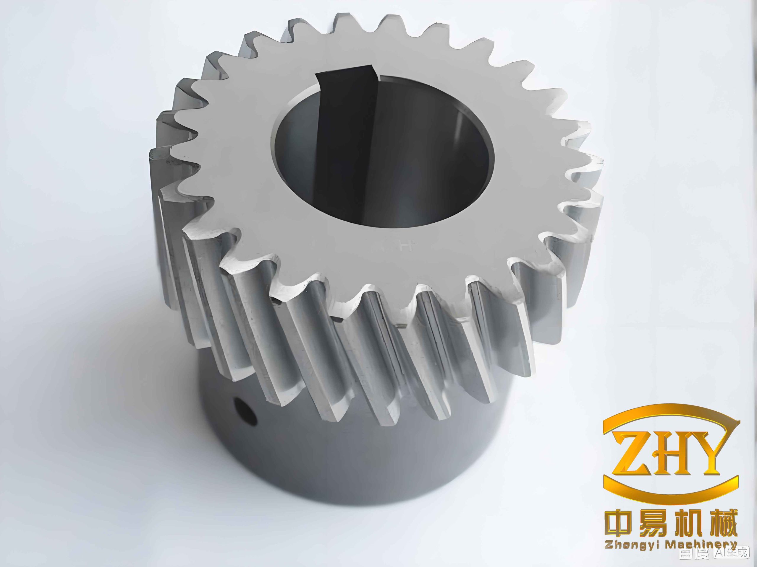
For the analytical mesh stiffness of helical gears, I used a slice-based energy accumulation method. I divided each helical gear into many thin slices along the face width. Each slice behaves approximately like a spur gear slice, but the contact position along the tooth profile changes as the contact line sweeps across the meshing plane. I calculated the local stiffness of each slice from bending, shear, radial compression, Hertz contact, and gear body deformation. Then I accumulated the contributions of all active slices along the actual contact lines. This allowed me to represent the helical gears with a stiffness model that retains the influence of contact ratio, helix angle, face width, and load position.
I expressed the total stiffness of a single slice at a contact point as the series combination of the compliance contributions of the two helical gears and the local contact. The total compliance of one meshing slice is
$$ \frac{1}{K_{\text{slice}}}=\frac{1}{k_b^p}+\frac{1}{k_b^g}+\frac{1}{k_s^p}+\frac{1}{k_s^g}+\frac{1}{k_a^p}+\frac{1}{k_a^g}+\frac{1}{k_h}+\frac{1}{k_f^p}+\frac{1}{k_f^g}. $$
Here \(k_b\), \(k_s\), \(k_a\), \(k_h\), and \(k_f\) are the bending, shear, axial compression, Hertz contact, and gear body stiffnesses. The superscripts \(p\) and \(g\) denote the driving and driven helical gears. I obtained the bending, shear, and axial compliances by integrating the strain energy along the involute profile. For a slice with tooth thickness and height varying along the profile, the bending stiffness is
$$ \frac{1}{k_b}=\int_0^d \frac{\left[(d-x)\cos\alpha_1-h\sin\alpha_1\right]^2}{E I_x}\,dx, $$
the shear stiffness is
$$ \frac{1}{k_s}=\int_0^d \frac{6\cos^2\alpha_1}{5 G A_x}\,dx, $$
and the axial compression stiffness is
$$ \frac{1}{k_a}=\int_0^d \frac{\sin^2\alpha_1}{E A_x}\,dx. $$
In these expressions, \(E\) is the elastic modulus, \(G\) is the shear modulus, \(A_x\) is the cross-sectional area at a local position, \(I_x\) is the area moment of inertia, \(d\) is the distance from the load point to the root, and \(\alpha_1\) is the angle between the load and the tooth centerline. I used the involute geometry to convert the integration variable from a straight cantilever coordinate into the involute angle. This step was important because the tooth profile of helical gears is not a simple rectangular beam.
For the Hertz contact stiffness, I assumed that the local contact behavior remains nearly constant within the allowable contact stress range. I used
$$ k_h=\frac{\pi E b_0}{4(1-\nu^2)}, $$
where \(b_0\) is the effective contact width and \(\nu\) is Poisson’s ratio. For the gear body stiffness, I used a closed-form elastic ring approximation. The body flexibility of helical gears cannot be ignored because the fillet and web regions deform under load, and this deformation modifies the effective mesh stiffness. I included it as
$$ \frac{1}{k_f}=\frac{\cos^2\alpha_1}{E b}\left[L^*\left(\frac{\mu_f}{S_f}\right)^2+M^*\left(\frac{\mu_f}{S_f}\right)+P^*\left(\frac{\mu_f}{S_f}\right)+Q^*\right], $$
where \(\mu_f\), \(S_f\), and the coefficients \(L^*\), \(M^*\), \(P^*\), and \(Q^*\) depend on the root geometry. The resulting single-slice mesh stiffness is
$$ k_{\text{slice}}(\alpha_1)=\left(\frac{1}{k_b^p}+\frac{1}{k_b^g}+\frac{1}{k_s^p}+\frac{1}{k_s^g}+\frac{1}{k_a^p}+\frac{1}{k_a^g}+\frac{1}{k_h}+\frac{1}{k_f^p}+\frac{1}{k_f^g}\right)^{-1}. $$
I validated the slice stiffness against an ISO-type constant stiffness estimate and a finite element contact model. The ISO method gives a useful average value but cannot reproduce the position-dependent variation. The finite element contact model gives high accuracy but requires much more computation. My analytical slice model retained most of the finite element trend and required only a small fraction of the computation time, which was essential because I later used it inside a multi-objective optimization loop.
| Parameter | Driving helical gear | Driven helical gear |
|---|---|---|
| Number of teeth | 53 | 63 |
| Normal module (mm) | 2.0 | 2.0 |
| Pressure angle (deg) | 14.5 | 14.5 |
| Helix angle (deg) | 27 | 27 |
| Face width (mm) | 20 | 20 |
| Total contact ratio | 3.0 | 3.0 |
For the contact line evolution of helical gears, I built a meshing plane coordinate system. In this plane, each tooth pair contact appears as a straight line inclined by the base helix angle. As the helical gears rotate, the contact line translates across the meshing plane. The number of active contact lines and their lengths depend on the transverse contact ratio and the overlap contact ratio. I separated the behavior into three cases: transverse contact ratio less than overlap contact ratio, equal contact ratios, and transverse contact ratio greater than overlap contact ratio. For the gear set I studied, the transverse contact ratio exceeded the overlap contact ratio, so the contact line length varied in three stages during one mesh cycle.
I discretized the meshing plane into a grid. The profile direction was divided into \(n\) positions, and the face width direction was divided into \(m\) slices. Each grid point represented a potential contact point. If a point lay inside the active contact line, I assigned the corresponding slice stiffness; otherwise, the contribution was zero. The total mesh stiffness of the helical gears at a time instant became
$$ K(t)=\sum_{j=1}^{m}\sum_{i=1}^{n} k_{ij}\Delta y \cos\beta_b, $$
where \(k_{ij}\) is the local slice stiffness at grid point \((i,j)\), \(\Delta y\) is the spacing along the contact line, and \(\beta_b\) is the base helix angle. Because several teeth can contact simultaneously, I summed the contributions of the first, second, and third active tooth pairs:
$$ K(t)=K^{I}(t)+K^{II}(t)+K^{III}(t). $$
This energy accumulation method allowed me to include the influence of helical gear geometry without using a full three-dimensional finite element model for every optimization iteration. I found that when the number of slices exceeded a moderate value, the mesh stiffness curve converged. For the helical gears in this transmission, forty slices along the face width were sufficient for the optimization, while a finer grid was used for final verification.
After obtaining the mesh stiffness, I built the static transmission error model. In a loaded gear pair, the actual meshing position differs from the ideal rigid-body position because of elastic deformation, manufacturing error, misalignment, and modification. I defined the transmission error at a contact point as
$$ \delta_{ij}=u_{ij}-\epsilon_{ij}, $$
where \(u_{ij}\) is the loaded deformation at the contact point and \(\epsilon_{ij}\) is the initial gap. The initial gap contains manufacturing error, backlash, profile modification, and lead modification:
$$ \epsilon_{ij}=\epsilon_{ij}^{m}+e_{ij}+x_{pm,ij}+x_{am,ij}. $$
For a given contact point, contact occurs only when \(\delta_{ij}>0\). The total mesh force must balance the external load:
$$ P=\sum_{i,j} k_{ij}\delta_{ij}=F. $$
I solved this nonlinear contact problem iteratively. I initialized the transmission error, computed the deformation at every grid point, set negative deformations to zero, summed the contact forces, and updated the transmission error until the load balance converged. The update rule was
$$ \delta^{(k+1)}=\delta^{(k)}-\frac{P^{(k)}-F}{k_s}, $$
where \(k_s\) is an average mesh stiffness. This iteration is simple but robust for the helical gears contact problem because the contact state is updated explicitly at every step.
I verified the transmission error model and the contact load distribution against a commercial finite element contact solver under three torque levels: 10 N·m, 100 N·m, and 200 N·m. The trends of transmission error and contact load matched closely. The peak-to-peak transmission error increased with torque, and the maximum contact load moved along the profile in the same way as the finite element result. The differences remained below the micron level for transmission error and below a few newtons per millimeter for contact load, which was acceptable for the subsequent robust optimization.
| Torque (N·m) | Analytical peak-to-peak TE (µm) | Finite element peak-to-peak TE (µm) | Maximum difference (µm) |
|---|---|---|---|
| 10 | 0.019 | 0.022 | 0.025 |
| 100 | 0.184 | 0.208 | 0.092 |
| 200 | 0.361 | 0.394 | 0.089 |
| Torque (N·m) | Analytical maximum contact load (N/mm) | Finite element maximum contact load (N/mm) | Difference (N/mm) |
|---|---|---|---|
| 10 | 3.61 | 3.63 | 0.02 |
| 100 | 35.9 | 37.2 | 1.3 |
| 200 | 71.6 | 74.3 | 2.7 |
I then studied how contact ratio and torque affect the transmission error of helical gears. When the total contact ratio was fixed and the transverse contact ratio varied from 1.2 to 1.8, both the mean transmission error and the peak-to-peak transmission error first decreased and then increased. The minimum occurred near a transverse contact ratio of 1.6. This trend appeared because the load sharing among tooth pairs changes with contact ratio. A very small contact ratio increases the load per tooth pair, while a very large contact ratio can create unfavorable phase relationships among the overlapping contact lines. When the transverse contact ratio was fixed and the overlap contact ratio increased from 1.0 to 1.6, both the mean and peak-to-peak transmission error decreased almost linearly. A larger overlap contact ratio means that the helical gears maintain a longer total contact line and smoother load transfer.
| Transverse contact ratio | Mean TE (µm) | Peak-to-peak TE (µm) | Trend |
|---|---|---|---|
| 1.2 | 0.74 | 0.43 | Higher |
| 1.4 | 0.51 | 0.31 | Decreasing |
| 1.6 | 0.38 | 0.20 | Minimum |
| 1.8 | 0.55 | 0.29 | Increasing |
| Overlap contact ratio | Mean TE (µm) | Peak-to-peak TE (µm) | Trend |
|---|---|---|---|
| 1.0 | 0.82 | 0.47 | Higher |
| 1.2 | 0.67 | 0.38 | Decreasing |
| 1.4 | 0.52 | 0.29 | Decreasing |
| 1.6 | 0.39 | 0.21 | Lower |
For torque influence, I found that without modification, both the mean transmission error and the peak-to-peak transmission error increased almost linearly with torque. This is expected because higher torque increases tooth deflection and contact load. With profile modification, the mean transmission error still increased with torque, but the increase became nonlinear and less steep after a certain torque. The peak-to-peak transmission error showed a more complex behavior: it first increased, then decreased, then increased again, and finally decreased. This behavior indicates that a fixed modification amount cannot be optimal for all torques. That observation motivated the robust optimization with torque variability.
I introduced profile modification and lead modification for the helical gears. Profile modification removes material near the tooth tip and root to compensate for elastic deflection and to reduce impact at the beginning and end of contact. I used a parabolic profile modification curve:
$$ H_a(y)=C_a\left(1-\frac{4y^2}{P_{bt}^2}\right), $$
where \(C_a\) is the profile modification amount, \(y\) is the coordinate along the profile, and \(P_{bt}\) is the base pitch. Lead modification changes the tooth surface along the face width to compensate for misalignment and to avoid edge contact. I used a linear lead modification curve:
$$ H_\beta(x)=G_\beta\frac{x\cos\beta}{b}, $$
where \(G_\beta\) is the lead modification amount, \(x\) is the coordinate along the face width, and \(b\) is the face width. By combining these two modification functions with the initial gap in the contact model, I obtained the modified transmission error model for helical gears.
I defined two objective functions. The first was the peak-to-peak transmission error, which represents the excitation level of the helical gears:
$$ f_{\text{PPTE}}=\delta_{\max}-\delta_{\min}. $$
The second was the maximum contact load, which represents the risk of concentrated contact and edge loading:
$$ f_{F\max}=\max\left(k_{ij}u_{ij}\right). $$
Because the transmission operates over a wide torque range, I treated torque as a random variable with a uniform probability density over a specified interval. I transformed each objective into a mean value:
$$ f_{i,\text{mean}}=\int_{T_l}^{T_u} f_i(x_{pm},x_{am},T)p_u(T)\,dT, $$
where the uniform density is
$$ p_u(T)=\frac{1}{T_u-T_l}. $$
This robust formulation prevents the optimization from selecting a modification that works only at one torque. I also included manufacturing roughness uncertainty. I represented surface roughness as a normal random variable,
$$ f(x)=\frac{1}{\sqrt{2\pi}\sigma}\exp\left[-\frac{(x-\mu)^2}{2\sigma^2}\right], $$
and I generated random errors for all contact grid points. The roughness perturbation changed the initial gap slightly at each contact point. By repeating the contact calculation with many random samples, I obtained a distribution of the objective functions rather than a single deterministic value.
I solved the robust multi-objective problem with the non-dominated sorting genetic algorithm III. I used the profile modification amount \(x_{pm}\) and the lead modification amount \(x_{am}\) as design variables. I bounded the profile modification from 0 to 20 µm and the lead modification from -20 to 20 µm. The fitness function combined the normalized robust objectives:
$$ F(x)=\min\left(\sum_{i=1}^{2}w_i f_i”(x_{pm},x_{am})\right)^2, $$
where \(f_i”\) is the normalized \(i\)-th objective and \(w_i\) is its weight. The algorithm generated reference points, performed non-dominated sorting, and selected individuals based on reference-point association. The final Pareto front contained a set of trade-off solutions between transmission error and contact load. From this front I selected four representative modification schemes plus the unmodified case for detailed comparison.
| Scheme | Profile modification (µm) | Lead modification (µm) | Peak-to-peak TE (m) | Maximum contact load (N/mm) |
|---|---|---|---|---|
| Unmodified | 0.0 | 0.0 | 0.18e-6 | 36.32 |
| Scheme I | 2.8 | 0.0 | 0.11e-6 | 41.81 |
| Scheme II | 6.7 | 0.0 | 0.06e-6 | 48.46 |
| Scheme III | 0.0 | 2.0 | 0.17e-6 | 31.04 |
| Scheme IV | 2.9 | 2.0 | 0.16e-6 | 36.80 |
I evaluated the modification schemes at 50 N·m and 200 N·m. At 50 N·m, the unmodified helical gears had a relatively smooth transmission error curve, but the peak-to-peak value was still significant. Scheme I produced the smallest peak-to-peak transmission error, while Scheme IV also reduced the fluctuation substantially. The contact load distribution became more uniform when lead modification was included. At 200 N·m, the unmodified helical gears had a larger mean transmission error and peak-to-peak value. Scheme II gave the smallest peak-to-peak transmission error, but it also produced the highest maximum contact load. Scheme IV gave a balanced result: it lowered the peak-to-peak transmission error compared with the unmodified case and kept the contact load distribution more uniform than Scheme II.
| Torque (N·m) | Scheme | Mean TE (µm) | Peak-to-peak TE (µm) | Maximum contact load (N/mm) |
|---|---|---|---|---|
| 50 | Unmodified | 1.38 | 0.103 | 18.2 |
| 50 | Scheme I | 2.27 | 0.006 | 25.2 |
| 50 | Scheme II | 3.12 | 0.071 | 32.6 |
| 50 | Scheme III | 0.38 | 0.084 | 18.7 |
| 50 | Scheme IV | 1.30 | 0.015 | 22.3 |
| 200 | Unmodified | 5.53 | 0.378 | 71.1 |
| 200 | Scheme I | 6.43 | 0.289 | 79.9 |
| 200 | Scheme II | 7.72 | 0.170 | 88.6 |
| 200 | Scheme III | 4.51 | 0.361 | 59.7 |
| 200 | Scheme IV | 5.47 | 0.273 | 64.8 |
I then constructed a fully coupled gear-bearing-rotor dynamic model. The model included the input shaft, the stationary housing shaft, the output shaft, the two helical gears, the angular contact ball bearings, the tapered roller bearings, and the housing foundation. I divided the shafts into Timoshenko beam elements. Each node had six degrees of freedom: three translations and three rotations. I assembled the element mass, stiffness, damping, and gyroscopic matrices into global matrices. The global equation of motion was
$$ \mathbf{M}\ddot{\mathbf{q}}+\left(\mathbf{C}+\mathbf{G}\right)\dot{\mathbf{q}}+\mathbf{K}\mathbf{q}=\mathbf{F}. $$
For the gear mesh element, I defined the displacement vector of the driving and driven helical gears as
$$ \mathbf{q}_s=\left[x_p,y_p,z_p,\theta_p,\phi_p,\psi_p,x_g,y_g,z_g,\theta_g,\phi_g,\psi_g\right]^T. $$
The relative deformation along the line of action was
$$ \sigma(t)=\mathbf{V}\mathbf{q}_s-e(t), $$
where \(e(t)\) is the static transmission error of the helical gears and \(\mathbf{V}\) is the projection vector. This vector contains the direction cosines of the mesh plane and the base radii of the two gears. The mesh force was obtained from the time-varying mesh stiffness and damping:
$$ F_m(t)=k(t)\sigma(t)+c(t)\dot{\sigma}(t). $$
I represented both the time-varying mesh stiffness and the transmission error as Fourier series. This step made the dynamic simulation efficient and allowed me to import the contact model results directly:
$$ k(t)=a_0+\sum_{n=1}^{N}\left[a_n\cos\left(\frac{2\pi n t}{T_m}\right)+b_n\sin\left(\frac{2\pi n t}{T_m}\right)\right], $$
$$ e(t)=c_0+\sum_{n=1}^{N}\left[c_n\cos\left(\frac{2\pi n t}{T_m}\right)+d_n\sin\left(\frac{2\pi n t}{T_m}\right)\right]. $$
I chose the Fourier order \(N=5\) because it captured the important harmonics of the helical gears while keeping the dynamic model compact. The mesh damping was related to the mesh stiffness by
$$ c(t)=2\xi\sqrt{\frac{k(t)m_p m_g}{m_p+m_g}}, $$
where \(\xi\) is the damping ratio. I used \(\xi=0.05\). I solved the global equation with the Newmark-\(\beta\) method. The method uses parameters \(\gamma_1=0.5\) and \(\beta_1=0.25\), which produce unconditional stability for linear systems and good accuracy for the periodic excitations of the helical gears.
| Scheme | c0 | c1 | d1 | c2 | d2 | c3 | d3 |
|---|---|---|---|---|---|---|---|
| Unmodified | 1.37e-6 | 4.63e-8 | 3.91e-9 | 8.14e-10 | 5.23e-9 | -1.92e-9 | 2.65e-10 |
| Scheme I | 2.27e-6 | -1.84e-9 | 7.41e-10 | -5.59e-10 | -1.26e-9 | 2.77e-10 | 2.14e-11 |
| Scheme II | 3.11e-6 | -3.23e-8 | -5.19e-9 | 2.56e-10 | 8.15e-9 | -2.50e-9 | -4.52e-10 |
| Scheme III | 8.76e-7 | 4.64e-8 | 5.33e-10 | 6.88e-10 | 3.40e-10 | -1.92e-9 | 1.98e-10 |
| Scheme IV | 7.78e-7 | 5.09e-9 | 8.95e-10 | 1.17e-10 | -1.69e-9 | -1.12e-9 | 1.34e-12 |
I calculated the natural frequencies of the coupled system with and without the housing shaft. Adding the housing shaft introduced thirty additional degrees of freedom and increased the flexibility of the input support. As a result, the natural frequencies decreased after the fourth mode, and new coupled modes appeared. This confirmed that the thin-walled housing shaft cannot be treated as rigid when predicting the vibration of the helical gears.
| Order | Without housing shaft (Hz) | With housing shaft (Hz) | Mode character |
|---|---|---|---|
| 1 | 522.1 | 520.9 | Output shaft bending-torsion |
| 2 | 1014.0 | 1010.3 | Input shaft bending-torsion |
| 3 | 1144.5 | 1144.5 | Input shaft axial-torsion |
| 4 | 1265.7 | 1144.8 | Input shaft axial-torsion |
| 5 | 1479.5 | 1265.0 | Bending-torsion |
| 6 | 1953.2 | 1478.2 | Output shaft bending-torsion |
| 7 | 2312.0 | 1942.0 | Bending-torsion-swing |
| 8 | 2512.5 | 2113.0 | Lateral translation |
| 9 | 2667.2 | 2302.1 | Bending-torsion |
| 10 | 2761.8 | 2384.3 | Lateral swing |
| 16 | 3250.5 | 2670.2 | Bending-torsion |
| 22 | 3672.1 | 3005.1 | Bending-torsion |
| 27 | 4271.5 | 3497.4 | Bending-torsion-swing |
| 45 | 9705.6 | 8693.5 | Coupled bending-torsion-swing |
I analyzed the time-domain response of the driving and driven helical gears at 2000 rpm and 100 N·m. The radial displacement, velocity, and acceleration of the two gears had similar waveforms, but the driving gear had slightly larger amplitudes because its support path included the flexible housing shaft. The torsional response was also periodic with the mesh frequency. The response was not symmetric about zero because the mean torque imposed a static offset on the torsional coordinate. The dynamic model therefore reproduced the expected behavior of the helical gears under combined bending, torsion, axial, and swing motion.
I then studied the vibration response of the system over a speed range from 0 to 5000 rpm. I found resonance bands near 591 rpm, 3015 rpm, 3402 rpm, and 3960 rpm. These speeds corresponded to mesh frequency components that approached the natural frequencies of the coupled system. At 591 rpm, the first natural frequency was excited, and the response was dominated by output shaft bending-torsion. At higher speeds, the excitation of higher modes produced bending-torsion and bending-torsion-swing responses. The amplitude of the helical gears was larger than that of the bearings because the mesh point directly receives the internal excitation.
I compared the four modification schemes under 50 N·m and 200 N·m. At 50 N·m, the displacement amplitude in the line-of-action direction increased with speed for all schemes, and resonance bands appeared at the same speeds. Scheme II produced the largest off-resonance amplitude, while Schemes III and IV produced smaller amplitudes. At the resonance speeds, Scheme IV gave the lowest peak amplitude. In the frequency domain, the unmodified helical gears showed clear peaks at the mesh frequency and at two, three, four, and five times the mesh frequency. Scheme IV suppressed the higher harmonic peaks almost completely while keeping the main mesh peak low.
At 200 N·m, the same overall trend appeared. The off-resonance amplitudes of the five cases were closer because the higher load made the contact stiffer and reduced the relative influence of the modification. However, at resonance, Scheme IV still produced the lowest peak amplitude. In the frequency domain, the unmodified case had strong higher harmonics, while Scheme IV again reduced the second, third, fourth, and fifth harmonics. Based on the combined transmission error, contact load, and dynamic response, I selected Scheme IV as the final robust modification for the helical gears.
| Condition | Best scheme for low TE | Best scheme for low contact load | Best overall dynamic response |
|---|---|---|---|
| 50 N·m | Scheme I | Scheme III | Scheme IV |
| 200 N·m | Scheme II | Scheme III | Scheme IV |
I built an NVH test bench for the transmission. The bench included a driving dynamometer, an absorbing dynamometer, a data acquisition system, three-axis accelerometers, microphones, and a semi-anechoic enclosure. I placed accelerometers on the top and sides of the first reduction housing and microphones at one meter from the transmission. I used order tracking to identify the vibration and noise sources. In order tracking, the order is defined as
$$ O=\frac{f}{f_0}, $$
where \(f\) is the frequency of interest and \(f_0\) is the reference shaft rotation frequency. By sampling at constant angular increments, I could separate the mesh orders of the helical gears from other transmission orders. The mesh order of the first reduction stage was the most prominent order in the measured spectrum, which confirmed that the first reduction helical gears were the dominant source of the whine.
| Test | Load torque (N·m) | Speed range (rpm) | Gear | Duration (s) |
|---|---|---|---|---|
| 1 | 50 | 0–4500 | Third | 10 |
| 2 | 50 | 0–4500 | Third | 10 |
| 3 | 200 | 0–4500 | Sixth | 10 |
| 4 | 200 | 0–4500 | Sixth | 10 |
For the third gear condition, the unmodified case produced strong order noise at the mesh order and its second harmonic. The maximum noise level reached about 65 dB. The dynamic model predicted the same order pattern, with the largest displacement amplitude in the same speed range. After applying Scheme IV to the helical gears, the second-harmonic order noise decreased significantly, and the higher harmonics became weak. The maximum noise level dropped to about 59 dB, which is an overall reduction of about 11%. The order slice at the mesh order showed that the modified case had a lower average level than the unmodified case across the speed range, with a reduction of about 14%.
| Third gear | Unmodified | Scheme IV | Change |
|---|---|---|---|
| Maximum noise level (dB) | 65 | 59 | −11% |
| Mesh order slice average | Reference | Lower | −14% |
| Higher harmonics | Strong | Weak | Suppressed |
For the sixth gear condition, the unmodified case produced even stronger order noise. The maximum level reached about 71 dB. The mesh order, second harmonic, and third harmonic were all visible. After applying Scheme IV, the second and third harmonics became much weaker, and the maximum noise level dropped to about 67 dB. This is an overall reduction of about 9%. The order slice at the higher harmonic showed a reduction of about 21% in average level. The experimental results therefore agreed with the dynamic model, which predicted that Scheme IV would reduce the higher harmonic components of the helical gears while maintaining a low main mesh peak.
| Sixth gear | Unmodified | Scheme IV | Change |
|---|---|---|---|
| Maximum noise level (dB) | 71 | 67 | −9% |
| Higher harmonic order slice average | Reference | Lower | −21% |
| Main mesh order | Strong | Reduced | Improved |
I concluded that the robust modification of the helical gears reduced the transmission error excitation, improved the contact load distribution, and lowered the order noise of the first reduction stage. The analytical mesh stiffness model provided the necessary speed and accuracy for optimization. The robust objective function prevented a torque-specific solution and produced a modification that worked under both low and high load. The coupled gear-bearing-rotor model showed why the housing shaft flexibility must be included: it shifts natural frequencies and creates additional coupled modes that can be excited by the helical gears. The order-tracking experiments confirmed the numerical predictions and showed that the selected modification reduced the third-gear noise by about 11% and the sixth-gear noise by about 9%. The same approach can be extended to other helical gears in the transmission, and additional objectives such as bearing load or housing radiation can be included in future robust optimization studies.