
I investigate the surge phenomenon that occurs in oil-lubricated helical gears under high-speed and heavy-load conditions. In my analysis, helical gears are not only power transmission components but also tribological systems in which the lubricant film, the solid tooth surface, and the dynamic meshing force interact continuously. When two tooth surfaces collide during meshing, the contact speed changes abruptly, and the lubricant film can enter an unstable state characterized by repeated oscillations. I refer to this unstable state as surge in helical gears. The occurrence of surge increases wear, reduces service life, and may induce alternating stresses that lead to fatigue cracks or even fracture. Therefore, I establish a coupled model that links the surge mechanism, elastohydrodynamic lubrication, and the nonlinear dynamics of helical gears.
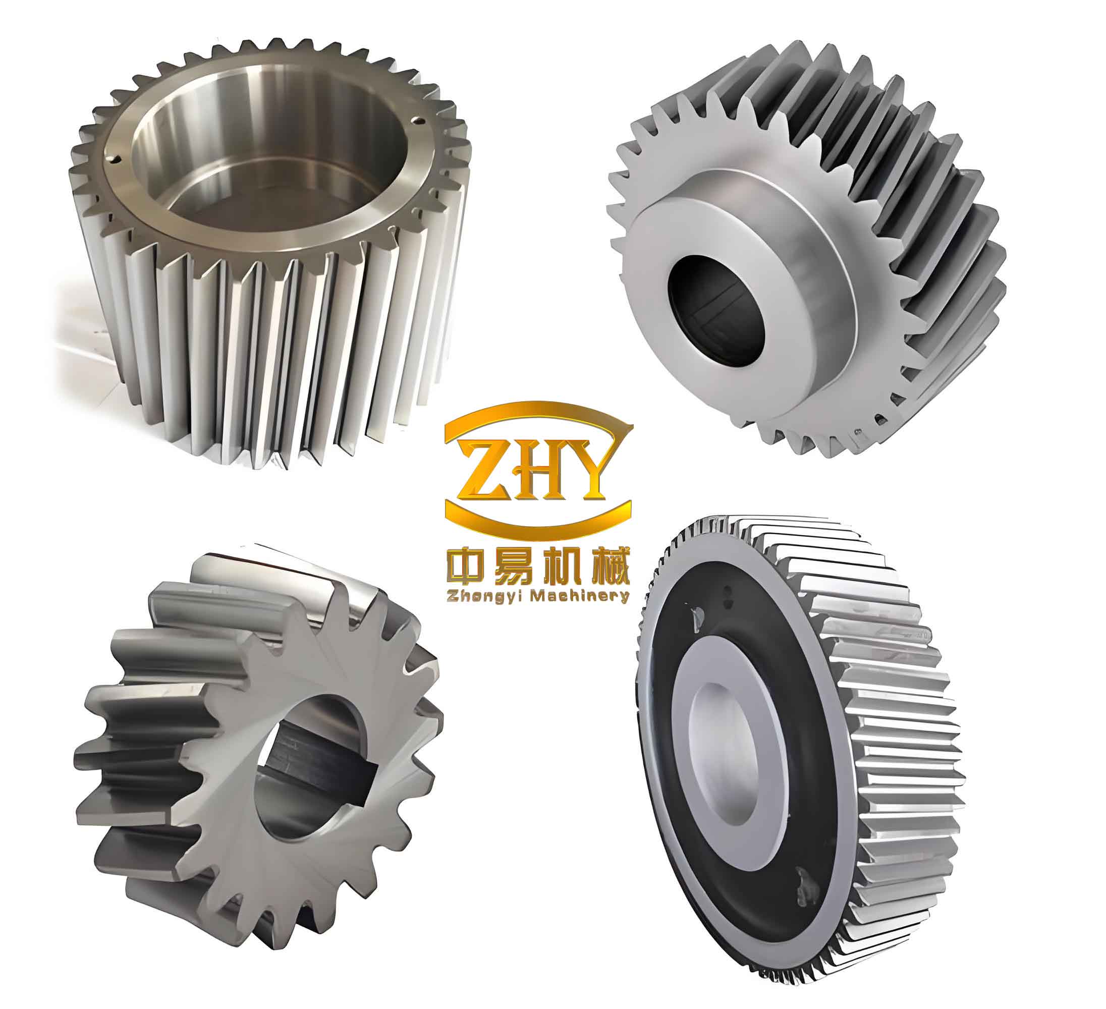
My starting point is the meshing impact of helical gears. Because of manufacturing and assembly errors, tooth profile deviations, and elastic deformation under load, the meshing point of a helical gear pair does not always lie exactly on the theoretical line of action. The driven gear tooth tip may contact the driving gear flank before the ideal meshing position, producing a corner contact and a normal impact velocity. I calculate the impact point by solving the geometric relations of the involute helical gears. The impact point radius on the driving gear is obtained from
$$
\rho_{O_1D} = \sqrt{r_{a2}^2 + a^2 – 2 r_{a2} a \cos(\theta_2 + \gamma_2)}
$$
where \(r_{a2}\) is the addendum circle radius of the driven gear, \(a\) is the center distance, \(\theta_2\) is the reversal angle of the driven gear, and \(\gamma_2\) is an auxiliary angle. The corresponding pressure angle at the impact point is
$$
\alpha_{D1} = \arccos\left(\frac{r_{b1}}{\rho_{O_1D}}\right)
$$
with \(r_{b1}\) being the base circle radius of the driving gear. The load distribution along the contact line of helical gears changes periodically. I use the contact-line percentage method to determine the distributed load. For a helical gear pair, the total contact line length is the sum of the individual contact line lengths of all meshing tooth pairs:
$$
l = \sum_{i=1}^{N} l_i
$$
The distributed load per unit contact line length is then
$$
F = \frac{F_t}{l \cos\alpha_t \cos\beta_b}
$$
where \(F_t\) is the tangential force, \(\alpha_t\) is the transverse pressure angle, and \(\beta_b\) is the base helix angle. This load distribution is essential because it directly affects the oil film pressure and the dynamic meshing force in helical gears.
I now model the solid-liquid interface slip. Under high-speed and heavy-load conditions, the shear stress at the interface between the lubricant and the tooth surface can exceed a limiting value. When this happens, the lubricant near the solid surface slips, and the velocity profile becomes discontinuous. The slip layer has a different effective viscosity from the central layer. I define the viscosity ratio \(\theta\) and the thickness ratio \(k\) as
$$
\theta = \frac{\eta_{\text{slip}}}{\eta_{\text{central}}}, \qquad k = \frac{h_1}{h_2}
$$
where \(h_1\) and \(h_2\) are the thicknesses of the upper and lower slip layers. The shear stress in each layer is balanced according to
$$
\frac{\partial p}{\partial x} = \frac{\partial \tau_{xz}}{\partial z}, \qquad
\frac{\partial p}{\partial y} = \frac{\partial \tau_{yz}}{\partial z}
$$
After integrating the velocity across the film thickness, I obtain the volume flow rate in the \(x\)-direction as
$$
q_x = \int_{0}^{h_1} u_1 dz + \int_{h_1}^{h-h_2} u_m dz + \int_{h-h_2}^{h} u_2 dz
$$
The same procedure gives the \(y\)-direction flow rate \(q_y\). These flow rates are then introduced into the modified Reynolds equation for surge in helical gears. The conventional Reynolds equation is
$$
\frac{\partial}{\partial x}\left(\frac{\rho h^3}{\eta}\frac{\partial p}{\partial x}\right)
+
\frac{\partial}{\partial y}\left(\frac{\rho h^3}{\eta}\frac{\partial p}{\partial y}\right)
=
12\frac{\partial(\rho h \bar{u})}{\partial x}
+
12\frac{\partial(\rho h \bar{v})}{\partial y}
+
\frac{\partial(\rho h)}{\partial t}
$$
For surge conditions, I introduce a backflow coefficient \(\lambda\), which is defined as the ratio of the backflow film thickness to the central film thickness:
$$
\lambda = \frac{h_{c,\text{back}}}{h_c}
$$
The modified Reynolds equation for helical gears under surge becomes
$$
\frac{\partial}{\partial x}\left(\frac{\rho h^3}{\eta}\frac{\partial p}{\partial x}\right)
+
\frac{\partial}{\partial y}\left(\frac{\rho h^3}{\eta}\frac{\partial p}{\partial y}\right)
=
\frac{\partial}{\partial x}\left[
\rho h (u_2 + u_1)(\lambda_s + \lambda_F)
\right]
+
\frac{\partial}{\partial y}\left[
\rho h (v_2 + v_1)(\lambda_s + \lambda_F)
\right]
$$
where \(\lambda_s\) and \(\lambda_F\) are coefficients derived from the slip layer and the backflow layer. The film thickness equation for helical gears is
$$
h(x,y) = h_0 + \frac{x^2}{2R} + \frac{2}{\pi E’}
\iint_{\Omega}
\frac{p(x’,y’)}{\sqrt{(x-x’)^2+(y-y’)^2}}
dx’dy’
$$
Here \(h_0\) is the rigid body displacement, \(R\) is the equivalent radius of curvature, and \(E’\) is the equivalent elastic modulus. I use the Ree-Eyring non-Newtonian model for the lubricant. The equivalent viscosity is
$$
\eta^* = \frac{\eta_0}{\tau_0 / \tau_e} \sinh\left(\frac{\tau_e}{\tau_0}\right)
$$
where \(\tau_0\) is the characteristic shear stress and \(\tau_e\) is the equivalent shear stress. The viscosity-pressure relation is
$$
\eta = \eta_0 \exp\left\{
\left(\ln\eta_0 + 9.67\right)
\left[
\left(1 + 5.1 \times 10^{-9} p\right)^Z – 1
\right]
\right\}
$$
The density-pressure relation is
$$
\rho = \rho_0
\left[
1 + \frac{0.6 \times 10^{-9} p}{1 + 1.7 \times 10^{-9} p}
\right]
$$
The load balance equation is
$$
w = \iint_{\Omega} p(x,y) dx dy
$$
To solve these equations, I nondimensionalize them and apply a multigrid method. The computational domain is divided into five grid levels. The finest level has 129 nodes in the \(X\)-direction and 513 nodes in the \(Y\)-direction. The pressure is solved using a Gauss-Seidel iteration, and the load balance is satisfied by adjusting the rigid body displacement. I use the following convergence criteria:
$$
\varepsilon_P = 10^{-5}, \qquad \varepsilon_F = 10^{-4}
$$
I verify my surge model by comparing the central film thickness and the minimum film thickness at the single-tooth meshing-in point, the pitch point, and the single-tooth meshing-out point. The results show that when the impact speed increases, the film thickness mutation becomes larger and the oscillation frequency decreases. This behavior confirms that surge in helical gears is strongly dependent on the impact speed and the impact position.
| Parameter | Value |
|---|---|
| Number of teeth, driving gear | 25 |
| Number of teeth, driven gear | 46 |
| Normal module, \(m_n\) | 3 mm |
| Normal pressure angle | 20° |
| Face width, \(B\) | 30 mm |
| Helix angle, \(\beta\) | 14° |
| Input speed | 1500 rpm |
| Input torque | 300 N·m |
The dynamic excitation of helical gears includes transmission error and time-varying meshing stiffness. I express the transmission error as a Fourier series. When only the first harmonic is retained, the transmission error is
$$
e(t) = e_1 \cos(\omega t)
$$
where \(e_1\) is the first harmonic amplitude and \(\omega\) is the meshing frequency. For the time-varying meshing stiffness, I use a single-tooth stiffness function of the form
$$
K_i(q) = k_p \exp\left[
C \left(
\frac{q/P_{bt} – \varepsilon_a / 2}{1.125}
\right)^3
\right]
$$
where \(k_p\) is the stiffness at the pitch point, \(q\) is the displacement along the line of action, \(P_{bt}\) is the base pitch, and \(\varepsilon_a\) is the transverse contact ratio. The total meshing stiffness is the sum of the individual tooth pair stiffnesses:
$$
K(q) = \sum_{i=1}^{N} K_i(q)
$$
I also calculate the oil film stiffness. The oil film is treated as an elastic element, and its stiffness is obtained by integrating the pressure over the contact area:
$$
K_c = \sum_{i=1}^{n} \frac{p_i}{h_i} \Delta x
$$
Then I define the coupled comprehensive stiffness of a single tooth pair as
$$
K_{ti} = \frac{K_i(q) K_c}{K_i(q) + K_c}
$$
The total comprehensive stiffness for helical gears is
$$
K_t = \sum_{i=1}^{N} K_{ti}
$$
This comprehensive stiffness is used in the dynamic model. I establish a four-degree-of-freedom dynamic model for the helical gear pair. The model includes the radial, tangential, axial, and torsional directions. The equations of motion are
$$
m_1 \ddot{x}_1 + c_{1x}\dot{x}_1 + k_{1x}x_1 = -F_x
$$
$$
m_1 \ddot{y}_1 + c_{1y}\dot{y}_1 + k_{1y}y_1 = -F_y
$$
$$
m_1 \ddot{z}_1 + c_{1z}\dot{z}_1 + k_{1z}z_1 = F_z
$$
$$
I_1 \ddot{\theta}_1 = F_y r_1 + T_1
$$
$$
m_2 \ddot{x}_2 + c_{2x}\dot{x}_2 + k_{2x}x_2 = F_x
$$
$$
m_2 \ddot{y}_2 + c_{2y}\dot{y}_2 + k_{2y}y_2 = F_y
$$
$$
m_2 \ddot{z}_2 + c_{2z}\dot{z}_2 + k_{2z}z_2 = -F_z
$$
$$
I_2 \ddot{\theta}_2 + k_t \theta_2 = F_y r_2 – T_2
$$
The dynamic meshing forces in the \(x\), \(y\), and \(z\) directions are
$$
F_x = k_{mx}(x_1 – x_2 + y_1 \tan\beta + y_2 \tan\beta + r_1\theta_1 – r_2\theta_2 – e_x)
+
c_{mx}(\dot{x}_1 – \dot{x}_2 + \dot{y}_1 \tan\beta + \dot{y}_2 \tan\beta + r_1\dot{\theta}_1 – r_2\dot{\theta}_2 – \dot{e}_x)
$$
$$
F_y = k_{my}(y_1 + r_1\theta_1 – y_2 – r_2\theta_2 – e_y)
+
c_{my}(\dot{y}_1 + r_1\dot{\theta}_1 – \dot{y}_2 – r_2\dot{\theta}_2 – \dot{e}_y)
$$
$$
F_z = k_{mz}(z_1 – z_2 – y_1 \tan\beta + y_2 \tan\beta + r_1\theta_1 – r_2\theta_2 – e_z)
+
c_{mz}(\dot{z}_1 – \dot{z}_2 – \dot{y}_1 \tan\beta + \dot{y}_2 \tan\beta + r_1\dot{\theta}_1 – r_2\dot{\theta}_2 – \dot{e}_z)
$$
The stiffness components along the coordinate axes are related to the normal meshing stiffness \(k_m\) by
$$
k_{mx} = k_m \sin\beta, \qquad
k_{my} = k_m \cos\beta \cos\alpha_n, \qquad
k_{mz} = k_m \cos\beta \sin\alpha_n
$$
The damping components follow the same decomposition. I write the dynamic equations in matrix form:
$$
[M]\{\ddot{\delta}\} + [C]\{\dot{\delta}\} + [K]\{\delta\} = \{F\}
$$
where \(\{\delta\}\) is the displacement vector
$$
\{\delta\} = \{x_1, y_1, z_1, \theta_1, x_2, y_2, z_2, \theta_2\}^T
$$
I solve this dynamic model together with the surge lubrication model in an iterative manner. The dynamic meshing force is used as the input load for the elastohydrodynamic lubrication analysis. The oil film stiffness and the impact speed are then fed back into the dynamic model. The iteration continues until the relative error of the dynamic meshing force is less than \(10^{-3}\).
| Material parameter | Driving gear | Driven gear |
|---|---|---|
| Density (kg/m³) | 7800 | 7800 |
| Specific heat (J/kg·K) | 465 | 465 |
| Thermal conductivity (W/m·K) | 50 | 50 |
| Hardness (HRC) | 50 | 50 |
| Elastic modulus (GPa) | 206 | 206 |
| Poisson ratio | 0.3 | 0.3 |
| Surface roughness (μm) | 0.5 | 0.5 |
| Friction coefficient | 0.135 | 0.135 |
| Lubricant parameter | Symbol | Value |
|---|---|---|
| Initial viscosity (Pa·s) | \(\eta_0\) | 0.05 |
| Viscosity-pressure coefficient (m²/N) | \(\alpha\) | \(2.3 \times 10^{-8}\) |
| Viscosity-pressure exponent | \(Z\) | 0.5687 |
| Limiting shear stress coefficient | \(\Lambda_{\lim}\) | 0.091 |
| Density (kg/m³) | \(\rho\) | 810 |
I analyze the dynamic characteristics of helical gears with and without surge. The vibration velocity and vibration displacement in the radial, tangential, axial, and torsional directions are calculated. When surge is considered, the vibration amplitudes and frequencies increase significantly in all directions. The tangential and torsional directions are more sensitive because the dynamic meshing force and the torque directly act in these directions. The axial direction also shows a noticeable increase due to the helix angle. The radial direction has the smallest response. The sudden changes in vibration velocity indicate that surge in helical gears is a transient instability triggered by meshing impact and interface slip.
I also study the nonlinear characteristics of helical gears under surge. The dimensionless excitation frequency \(\omega\) is used as the control parameter. The bifurcation diagram shows that the system undergoes a sequence of periodic, multi-periodic, chaotic, and quasi-periodic motions. When \(\omega\) is small, the system is in a stable single-period state. As \(\omega\) increases, period-doubling bifurcations occur, and the system enters chaos. After a chaotic window, the system returns to periodic motion. The main bifurcation intervals are summarized in the following table.
| Dimensionless excitation frequency range | Dynamic behavior |
|---|---|
| \(\omega < 0.289\) | Stable single-period motion |
| \(0.289 < \omega < 0.327\) | Transition to period-2 motion |
| \(0.327 < \omega < 0.401\) | Period-2 and period-4 motion |
| \(0.401 < \omega < 0.436\) | Period-4 to chaos |
| \(0.436 < \omega < 1.474\) | Chaotic motion |
| \(1.474 < \omega < 1.767\) | Period-2 and quasi-periodic motion |
| \(1.767 < \omega < 2.618\) | Multi-periodic motion |
| \(\omega > 2.618\) | Stable single-period motion |
The Poincaré maps and phase portraits confirm the bifurcation results. When \(\omega = 0.2\), the phase portrait is a closed curve and the Poincaré map contains a finite number of points, indicating a stable periodic motion. When \(\omega = 0.55\), the Poincaré map contains a large number of scattered points, which is a signature of chaos. When \(\omega = 1.6\), the system shows multi-periodic behavior. When \(\omega = 1.767\), the system returns to a more regular motion. When \(\omega = 2.5\) and \(\omega = 2.6\), the system is again in a periodic state. These results show that increasing the excitation frequency can suppress surge in helical gears, while decreasing the error amplitude can also reduce the chaotic region.
I next investigate the effect of error amplitude on surge. The dimensionless load parameter is defined as the ratio of external excitation to internal error excitation. When the external excitation is fixed, a larger error amplitude corresponds to a smaller load parameter. The bifurcation diagram with respect to error amplitude shows that the system remains in a stable single-period state when the error amplitude is below 0.1366. Period-doubling occurs between 0.1366 and 0.1660. A period-4 motion appears between 0.1660 and 0.1894. The system returns to period-2 between 0.1894 and 0.2059. When the error amplitude exceeds 0.2059, the system enters chaos. Therefore, reducing the transmission error amplitude is an effective way to avoid surge in helical gears.
The load and torque also have a strong influence on surge. I calculate the oil film pressure and film thickness at the meshing-in point, the pitch point, and the meshing-out point under different torques. The results are summarized below.
| Contact point | Effect of increasing torque |
|---|---|
| Meshing-in point | Pressure increases; end leakage becomes more severe; film thickness changes slightly |
| Pitch point | Pressure oscillation amplitude increases; film thickness in the \(Y\)-direction increases; surge becomes more obvious |
| Meshing-out point | Pressure and film thickness increase; surge is amplified |
For load conditions, I compare light load, medium load, and heavy load. The central film thickness and minimum film thickness both decrease as the load increases. At the same time, the mutation amplitude of the film thickness increases. Heavy load therefore makes surge in helical gears more likely and more severe. This is because the higher contact pressure reduces the film thickness and increases the elastic deformation of the tooth surface, which in turn changes the effective contact geometry and the lubricant flow.
| Load condition | Central film thickness | Minimum film thickness | Surge severity |
|---|---|---|---|
| Light load | Largest | Largest | Weakest |
| Medium load | Medium | Medium | Moderate |
| Heavy load | Smallest | Smallest | Strongest |
I also analyze the influence of lubricant parameters. The initial viscosity and the viscosity-pressure coefficient are two key factors. For the initial viscosity, I compare values of 0.25 Pa·s, 0.35 Pa·s, and 0.45 Pa·s. The oil film pressure changes only slightly, but the film thickness increases with increasing initial viscosity. A higher initial viscosity increases the resistance of the lubricant to squeezing and enhances the load-carrying capacity of the film. As a result, surge in helical gears is weakened. The effect of the viscosity-pressure coefficient is similar. When the viscosity-pressure coefficient increases from 25 GPa\(^{-1}\) to 45 GPa\(^{-1}\) and then to 65 GPa\(^{-1}\), both the film pressure and the film thickness increase. The higher viscosity-pressure coefficient makes the lubricant viscosity rise more rapidly under high pressure, which increases the film thickness and improves the load capacity. Therefore, within a reasonable range, increasing either the initial viscosity or the viscosity-pressure coefficient can suppress surge in helical gears.
| Lubricant parameter | Variation | Effect on film thickness | Effect on surge |
|---|---|---|---|
| Initial viscosity | 0.25 → 0.45 Pa·s | Increases | Weakens |
| Viscosity-pressure coefficient | 25 → 65 GPa\(^{-1}\) | Increases | Weakens |
Based on these results, I propose several suppression strategies for surge in helical gears. First, the transmission error amplitude should be reduced by improving manufacturing accuracy, optimizing the tooth profile, and using appropriate tooth surface modification. Second, the excitation frequency should be adjusted by changing the gear ratio, the relative position of the gears, or the operating speed. Third, the load should be controlled so that the helical gears avoid heavy-load conditions that produce very thin films. Fourth, the lubricant should be selected with a suitable initial viscosity and viscosity-pressure coefficient to maintain a stable film. Fifth, the solid-liquid interface slip should be controlled by improving surface finish and selecting lubricants with appropriate limiting shear stress. These strategies can be combined to improve the stability of helical gears and reduce the risk of surge.
In my coupled model, the surge phenomenon in helical gears is treated as a feedback process. The meshing impact generates a sudden change in surface velocity. The velocity change modifies the entrainment speed and the backflow coefficient. The modified Reynolds equation then predicts a film thickness oscillation. The film thickness oscillation changes the oil film stiffness. The oil film stiffness changes the comprehensive meshing stiffness. The comprehensive meshing stiffness changes the dynamic meshing force. Finally, the dynamic meshing force changes the impact load and the contact velocity, closing the loop. This closed-loop interaction explains why surge in helical gears can persist and why it is sensitive to both operating conditions and lubricant properties.
I further examine the transformation from stable motion to surge and from surge back to stable motion. In the stable state, the film thickness and pressure fluctuate periodically with the meshing cycle. In the surge state, the film thickness shows a sharp increase followed by irregular oscillations. The pressure also shows large-amplitude oscillations, especially near the pitch point. When the operating conditions are adjusted so that the excitation frequency moves out of the chaotic window, the system returns to a stable periodic state. This return is not instantaneous but occurs through a sequence of period-doubling and quasi-periodic transitions. The ability to predict these transitions is important for condition monitoring and active control of helical gears.
The dynamic responses of the driving and driven gears are different. The driving gear is connected to the input torque, while the driven gear is connected to the load torque. The torsional vibration of the driving gear is dominated by the input torque fluctuation. The torsional vibration of the driven gear is dominated by the load torque and the meshing force. In both gears, the tangential direction and the torsional direction have larger vibration amplitudes than the radial and axial directions. When surge occurs, the torsional vibration velocity of the driving gear can increase by more than 40 percent compared with the stable state. The corresponding displacement also increases significantly. This result suggests that torsional vibration monitoring is a practical way to detect surge in helical gears.
The time-varying contact line length of helical gears plays an important role in surge. Because the contact line length changes continuously, the distributed load changes continuously. The oil film pressure therefore changes continuously even without surge. When surge occurs, the pressure oscillation is superimposed on this gradual variation. The pitch point is the most sensitive location because the sliding velocity is zero there, and the film is most vulnerable to squeeze motion. The meshing-in point and meshing-out point are also sensitive but to a lesser degree. This spatial sensitivity means that surge in helical gears is not uniformly distributed along the contact line.
I use the multigrid method to solve the elastohydrodynamic lubrication problem because it can handle the large range of length scales and the strong nonlinearity of the Reynolds equation. The pressure is solved on multiple grid levels, and the low-frequency error is eliminated on the coarse grids. The high-frequency error is eliminated on the fine grids. The W-cycle is used to accelerate convergence. The pressure at each time step is initialized with the pressure from the previous time step. This approach reduces the computational cost and improves the stability of the solution. The convergence of the coupled model is checked at every iteration by comparing the dynamic meshing force, the oil film stiffness, and the surge film thickness with their previous values.
For the dynamic model, I use the Runge-Kutta method to integrate the equations of motion. The time step is chosen small enough to capture the impact and the high-frequency oscillation. The dynamic meshing force is calculated at each time step and passed to the lubrication model. The lubrication model returns the oil film stiffness and the film thickness distribution. The comprehensive stiffness is then updated. This procedure is repeated until the relative error is less than the specified tolerance. The coupled model is computationally intensive, but it provides a more realistic prediction of surge in helical gears than uncoupled models.
My results show that surge in helical gears is not a single-frequency phenomenon. It contains a broad spectrum of frequencies because the impact, the interface slip, and the nonlinear dynamics all contribute. The dominant frequency is related to the meshing frequency, but there are also subharmonic and superharmonic components. The presence of multiple frequencies makes surge difficult to identify using simple frequency analysis. Time-frequency methods or nonlinear feature extraction methods are more suitable. In my analysis, the Poincaré map and the bifurcation diagram are effective tools for identifying the transition to chaos. The phase portrait shows the shape of the limit cycle or the chaotic attractor. These tools can be used in condition monitoring of helical gears.
The practical implications of my study are as follows. First, designers of helical gears should consider the coupled effect of meshing impact, interface slip, and dynamic load. Second, the lubricant should be selected not only for its viscosity at the operating temperature but also for its limiting shear stress and viscosity-pressure behavior. Third, the tooth surface finish should be controlled to delay the onset of interface slip. Fourth, the operating speed and load should be kept away from the chaotic regions identified in the bifurcation diagram. Fifth, the gear ratio and the center distance should be optimized to adjust the excitation frequency. These measures can reduce the risk of surge in helical gears and improve the reliability of the transmission system.
In conclusion, I have established a coupled surge-dynamics model for helical gears that includes meshing impact, solid-liquid interface slip, elastohydrodynamic lubrication, time-varying meshing stiffness, transmission error, and nonlinear dynamics. I have solved the model using a multigrid method and a Runge-Kutta method, and I have verified the surge model against known film thickness trends. I have shown that surge in helical gears is strongly influenced by impact speed, impact position, torque, load, initial viscosity, and viscosity-pressure coefficient. I have identified chaotic and periodic regions in the parameter space. I have proposed suppression strategies based on reducing transmission error, adjusting excitation frequency, controlling load, and optimizing lubricant properties. My study provides a theoretical basis for understanding and suppressing surge in helical gears.
The main conclusions can be summarized as follows. The meshing impact and the interface slip are the two key triggers of surge in helical gears. The pitch point is the most sensitive location for surge. The torsional and tangential directions are the most affected by surge. The nonlinear dynamics of helical gears under surge include period-doubling, chaos, and quasi-periodic motion. Increasing the excitation frequency and reducing the error amplitude are effective ways to suppress surge. Increasing the initial viscosity and the viscosity-pressure coefficient within a reasonable range can also weaken surge. Heavy load and high torque make surge more severe. These conclusions are useful for the design, operation, and maintenance of helical gears in high-speed and heavy-load applications.