
In this study, I investigated a helical gear pair used in an automotive transmission. My work combined parametric modeling, modal analysis, tooth profile modification, response surface methodology, transmission error verification, and nonlinear dynamic analysis. The main objective was to improve the running stability of helical gears, reduce mesh impact, and understand how important system parameters influence the nonlinear motion of helical gears under different load conditions. I used SolidWorks for parametric modeling, ANSYS Workbench for finite element simulation, Design Expert for response surface design, Romax for transmission error and load verification, and Matlab for numerical solution of the dynamic equations. The results show that a properly designed tooth profile modification can significantly reduce contact stress and transmission error, while the dynamic behavior of helical gears is strongly affected by load, mesh stiffness, damping, and backlash.
1. Parametric Modeling of Helical Gears
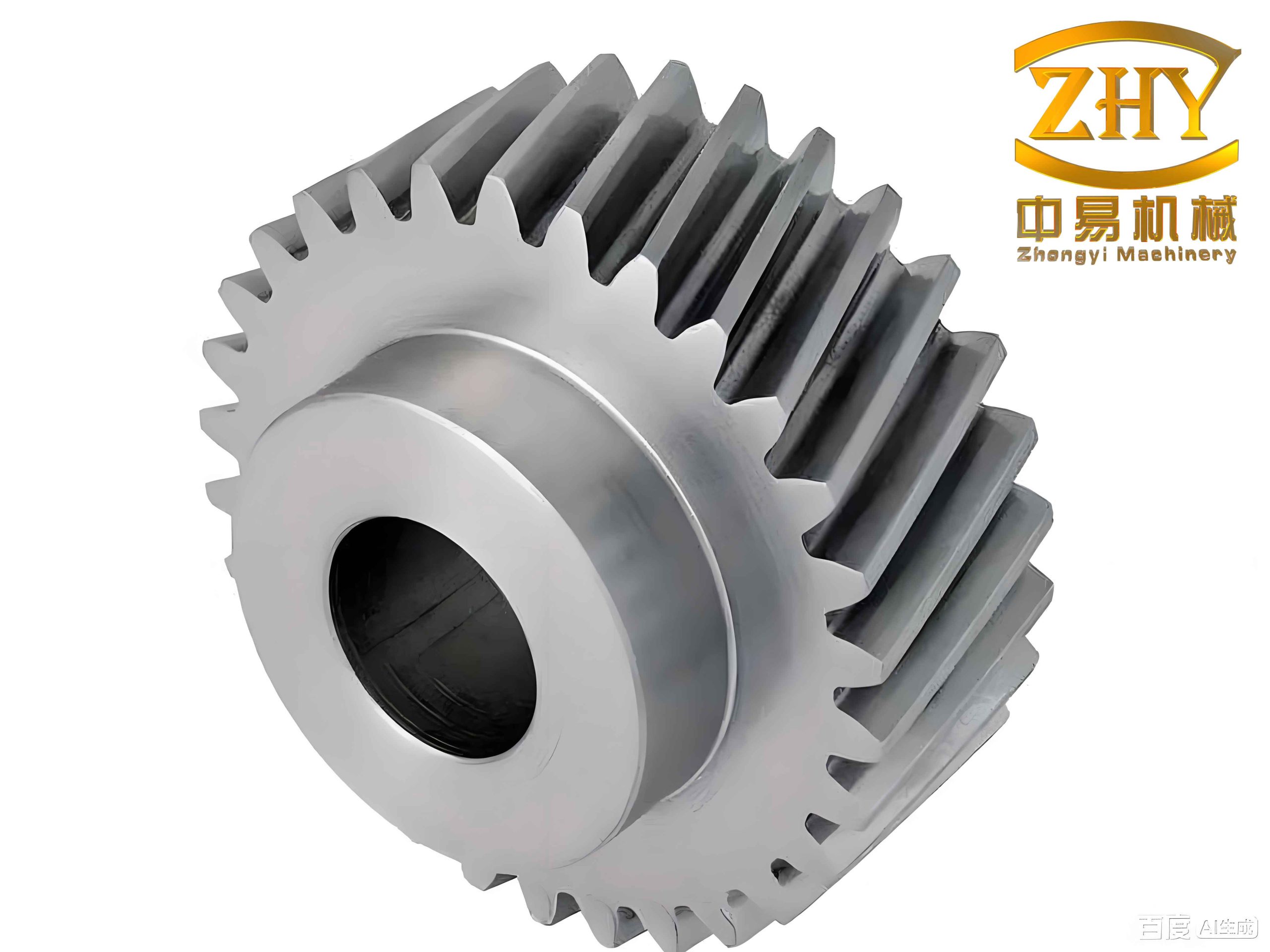
I began with a helical gear pair whose basic parameters are representative of an automotive transmission application. The two helical gears have opposite helix directions and the same normal module and normal pressure angle. In the transverse plane, the helical gears behave similarly to a spur gear pair, but the helix angle introduces axial contact and a gradual engagement process. The basic parameters I used are listed in Table 1.
| Parameter | Driving Gear | Driven Gear |
|---|---|---|
| Number of teeth | 23 | 44 |
| Helix angle (degree) | 16.835 | 16.835 |
| Pressure angle (degree) | 19 | 19 |
| Normal module (mm) | 4 | 4 |
| Face width (mm) | 24 | 22 |
| Pitch diameter (mm) | 96.1 | 183.9 |
The involute profile is the foundation of the tooth flank of helical gears. I generated the involute curve from the rolling motion of a straight line on a base circle. For a point on the involute, the coordinates in the Cartesian system can be written as follows:
$$ x = r_b(\cos u + u\sin u) $$
$$ y = r_b(\sin u – u\cos u) $$
Here, \(r_b\) is the base radius and \(u\) is the roll angle of the generating line. The base radius is related to the transverse pitch radius and the transverse pressure angle. For helical gears, the transverse pressure angle is different from the normal pressure angle because of the helix angle. I used the following relationship to determine the base radius:
$$ r_b = \frac{m_n z}{2\cos\beta}\cos\alpha_t $$
where \(m_n\) is the normal module, \(z\) is the number of teeth, \(\beta\) is the helix angle, and \(\alpha_t\) is the transverse pressure angle. The roll angle at the addendum circle is obtained from the addendum radius and the base radius:
$$ u_a = \sqrt{\left(\frac{r_a}{r_b}\right)^2 – 1} $$
With these equations, I created the involute profile in SolidWorks by using a parametric equation. I then generated the helical sweep along the helix line determined by the helix angle. After cutting a single tooth space, I patterned the tooth space around the gear axis to obtain the complete helical gear. I repeated the procedure for the mating gear by changing the number of teeth and the face width. The helical gear pair was then assembled with the correct center distance and helix directions.
For the modified tooth profile, I introduced a normal modification amount along the involute normal direction. If the original point on the involute is \(K(x,y)\), the modified point \(K'(x’,y’)\) can be expressed as:
$$ x’ = x – \Delta \sin(\alpha_k + \theta_k) $$
$$ y’ = y + \Delta \cos(\alpha_k + \theta_k) $$
where \(\Delta\) is the modification amount, \(\alpha_k\) is the pressure angle at point \(K\), and \(\theta_k\) is the involute angle at point \(K\). This formulation allowed me to build modified helical gears directly from the involute equation rather than relying on approximate geometric edits.
2. Modal Characteristics of the Helical Gear System
I performed modal analysis to determine the natural frequencies and mode shapes of the helical gear system. Modal analysis is important because it helps predict possible resonance conditions. If an excitation frequency coincides with a natural frequency of the helical gears, the vibration amplitude may increase sharply, which can reduce transmission accuracy and accelerate fatigue damage. The general equation of motion for a linear multi-degree-of-freedom system is:
$$ [M]\{\ddot{q}(t)\} + [C]\{\dot{q}(t)\} + [K]\{q(t)\} = \{F(t)\} $$
For free vibration, the external force and damping are neglected, so the equation becomes:
$$ [M]\{\ddot{q}(t)\} + [K]\{q(t)\} = 0 $$
The solution can be written as a superposition of modal contributions:
$$ q(t) = \sum_{r=1}^{n} C_r u^{(r)} \cos(\omega_r t – \psi_r) $$
Here, \(u^{(r)}\) is the modal vector, \(\omega_r\) is the natural frequency, \(C_r\) is a modal amplitude, and \(\psi_r\) is a phase angle. I imported the solid model into ANSYS Workbench and assigned the material properties. The material was 20CrMnTi, a common carburizing steel for transmission gears. The material properties I used are summarized in Table 2.
| Property | Value |
|---|---|
| Material | 20CrMnTi |
| Young modulus | 212 GPa |
| Poisson ratio | 0.289 |
| Density | 7860 kg/m3 |
| Contact friction coefficient | 0.2 |
I used tetrahedral elements with a multi-zone meshing method. The contact surfaces of the helical gears were refined to improve the accuracy of the contact solution. The driving gear tooth flank was set as the contact surface, and the driven gear tooth flank was set as the target surface. I used frictional contact with a coefficient of 0.2 and the augmented Lagrange algorithm. The boundary conditions were applied according to the actual working condition. The driven gear was loaded with a torque of 200 N m.
The first fifteen natural frequencies were extracted. The first natural frequency of the unmodified helical gear system was 3297.9 Hz, and the fifteenth natural frequency was 12544 Hz. The maximum mesh frequency under the operating speed was lower than the first natural frequency, which indicates that the helical gears in this transmission would not resonate under normal operating conditions. The mode shapes were dominated by torsional vibration, especially for the driven gear. The first and ninth modes mainly showed torsional vibration of the driven gear about the X axis, while the sixth mode showed torsional vibration of the driven gear about the Z axis. The first twelve modes were mainly related to the driven gear, whereas the thirteenth, fourteenth, and fifteenth modes were mainly related to the driving gear. After tooth profile modification, the first natural frequency increased to 3532.1 Hz, which is about 7.1 percent higher than that of the unmodified helical gears. This change indicates that tooth profile modification can slightly improve the structural dynamic stiffness of the helical gear system.
| Condition | First Natural Frequency (Hz) | Change |
|---|---|---|
| Unmodified helical gears | 3297.9 | Reference |
| Modified helical gears | 3532.1 | +7.1% |
3. Tooth Profile Modification of Helical Gears
Tooth profile modification is one of the most effective methods for reducing mesh impact and improving the running stability of helical gears. During meshing, the load is not constant. The contact ratio of helical gears is larger than that of spur gears, and the load distribution changes gradually along the contact line. However, manufacturing errors, assembly errors, and elastic deformation can still cause sudden changes in the normal pitch. These changes may produce meshing interference at the beginning and end of contact, which increases vibration and noise. Tooth profile modification removes a small amount of material near the tooth tip or tooth root so that the loaded tooth pair can enter and leave mesh more smoothly.
There are two main categories of gear modification: profile modification and lead modification. Profile modification changes the tooth profile in the transverse plane, while lead modification changes the tooth surface along the face width direction. The main methods and their functions are summarized in Table 3.
| Modification Type | Typical Method | Main Effect |
|---|---|---|
| Profile modification | Tip relief, root relief, root trimming | Reduces mesh impact and interference |
| Lead modification | Crowning, helix angle correction, end relief | Improves load distribution along face width |
| Combined modification | Profile and lead modification together | Improves both engagement and load distribution |
In my study, I focused on tooth profile modification of helical gears. The main design parameters are the modification curve, the maximum modification amount, and the modification length. The modification curve determines how the modification amount varies from the start of modification to the tooth tip. A parabolic curve is widely used because it can approximate the elastic deformation curve of the tooth pair. I used the following parabolic modification curve:
$$ \Delta_x = \Delta_{\max}\left[(1-a)\left(\frac{x}{L}\right)^2 + a\left(\frac{x}{L}\right)\right] $$
Here, \(\Delta_{\max}\) is the maximum modification amount, \(L\) is the modification length, \(x\) is the position along the modification region, and \(a\) is the curve coefficient. When \(a=0\), the curve is purely parabolic. When \(a=1\), the curve becomes linear. I also considered an exponential modification curve:
$$ \Delta_x = \Delta_{\max}\left(\frac{x}{L}\right)^n $$
where \(n\) is the exponent. A circular arc modification curve can also be used. For an arc modification, the modification amount is expressed as:
$$ \Delta_x = \frac{d}{2} – \sqrt{\frac{d^2}{4} – \frac{x^2}{\cos^2\alpha}} $$
The maximum modification amount must be selected carefully. If it is too small, the interference is not fully removed. If it is too large, the contact ratio decreases and the tooth strength is weakened. Several empirical formulas are available. The ISO formula for maximum modification amount is:
$$ \Delta_{\max} = \frac{K_A F_t}{b C_\gamma \varepsilon_\alpha} $$
where \(K_A\) is the application factor, \(F_t\) is the tangential force, \(b\) is the face width, \(C_\gamma\) is the comprehensive mesh stiffness, and \(\varepsilon_\alpha\) is the transverse contact ratio. The H. Sigg formulas for helical gears are:
$$ \Delta_{\max 1} = 4 + 0.04\frac{F_t}{b} \pm 4 $$
$$ \Delta_{\max 2} = 9 + 0.04\frac{F_t}{b} \pm 3.5 $$
The Walker method relates the maximum modification amount to the deflection at the highest point of single tooth contact. The maximum modification amount for the driving gear tip is:
$$ \Delta_A = \delta_{1B} + \delta_{2B} $$
and for the driven gear tip:
$$ \Delta_E = \delta_{1D} + \delta_{2D} $$
where \(\delta_{1B}\) and \(\delta_{2B}\) are the deflections of the two gears at point B, and \(\delta_{1D}\) and \(\delta_{2D}\) are the deflections at point D. In practice, manufacturing errors should also be included. The total modification amount can be written as:
$$ \Delta = \delta + \Delta m $$
where \(\Delta m\) is the manufacturing error. For helical gears, the modification length can be determined by either the long modification method or the short modification method. The long modification method is suitable for helical gears with large helix angle and large axial contact ratio. The short modification method is suitable for spur gears or helical gears with small helix angle. In my study, I used tip relief for both gears and distributed the modification amount between the driving and driven gears to avoid excessive weakening of the tooth thickness.
4. Response Surface Analysis for Tooth Profile Modification
To consider the combined influence of the main modification parameters, I used response surface methodology. This method designs a set of experiments, fits a regression model between the factors and the responses, and then finds the optimal factor combination. I selected three factors: the maximum modification amount \(A\), the modification length \(B\), and the modification curve coefficient \(C\). Before the formal response surface design, I used a control variable method with ANSYS Workbench to determine reasonable ranges for these factors. The ranges are given in Table 4.
| Factor | Symbol | Range |
|---|---|---|
| Maximum modification amount | A | 20 to 70 micrometer |
| Modification length | B | 3 to 7 mm |
| Modification curve coefficient | C | 0.2 to 0.8 |
The response values were the maximum equivalent elastic strain \(R_1\), with units of mm/mm, and the maximum equivalent stress \(R_2\), with units of MPa. I used the Box-Behnken design method to arrange the experiments. The design matrix and the finite element results are shown in Table 5.
| Run | A | B | C | R1 | R2 |
|---|---|---|---|---|---|
| 1 | 20 | 5 | 0.8 | 0.0033674 | 647.25 |
| 2 | 45 | 3 | 0.2 | 0.0032746 | 616.43 |
| 3 | 45 | 5 | 0.5 | 0.0030715 | 537.52 |
| 4 | 45 | 5 | 0.5 | 0.0030784 | 551.77 |
| 5 | 70 | 7 | 0.5 | 0.0034018 | 697.83 |
| 6 | 70 | 3 | 0.5 | 0.0034415 | 726.37 |
| 7 | 70 | 5 | 0.2 | 0.0033305 | 626.48 |
| 8 | 45 | 3 | 0.8 | 0.0033227 | 629.21 |
| 9 | 70 | 5 | 0.8 | 0.0034002 | 658.39 |
| 10 | 45 | 5 | 0.5 | 0.0030732 | 541.22 |
| 11 | 45 | 7 | 0.2 | 0.0032407 | 585.18 |
| 12 | 20 | 7 | 0.5 | 0.0033926 | 682.46 |
| 13 | 20 | 3 | 0.5 | 0.0034379 | 702.94 |
| 14 | 45 | 5 | 0.5 | 0.0030793 | 556.35 |
| 15 | 45 | 7 | 0.8 | 0.0032415 | 602.47 |
| 16 | 45 | 5 | 0.5 | 0.0030778 | 548.28 |
| 17 | 20 | 5 | 0.2 | 0.0033207 | 623.72 |
Using the Box-Behnken results, I fitted quadratic response surface models. The general form of the response surface model is:
$$ R = \beta_0 + \sum_{i=1}^{n}\beta_i x_i + \sum_{i=1}^{n}\beta_{ii}x_i^2 + \sum_{i<j}\beta_{ij}x_i $$=""
For the equivalent elastic strain \(R_1\), the model showed a high coefficient of determination. The determination coefficient was 0.9973, the adjusted coefficient was 0.9939, the predicted coefficient was 0.9595, and the signal-to-noise ratio was 44.3432. For the equivalent stress \(R_2\), the determination coefficient was 0.9932, the adjusted coefficient was 0.9844, the predicted coefficient was 0.9481, and the signal-to-noise ratio was 30.4719. These values indicate that the response surface models were accurate enough for design optimization. The fit statistics are summarized in Table 6.
| Response | R2 | Adjusted R2 | Predicted R2 | Signal-to-Noise Ratio |
|---|---|---|---|---|
| R1 | 0.9973 | 0.9939 | 0.9595 | 44.3432 |
| R2 | 0.9932 | 0.9844 | 0.9481 | 30.4719 |
The response surfaces showed that the maximum modification amount and the modification length had a strong influence on both the equivalent elastic strain and the equivalent stress. When the maximum modification amount increased from 20 micrometer to about 45 micrometer, the stress decreased. When it increased further toward 70 micrometer, the stress increased again. A similar trend was observed for the modification length. The curve coefficient had a smaller effect, but a value near 0.4 gave a relatively low stress. Based on the optimization, the best combination was a maximum modification amount of about 44.5 micrometer, a modification length of about 5.2 mm, and a curve coefficient of about 0.4. With this combination, the predicted maximum equivalent elastic strain was 0.0030802 mm/mm and the predicted maximum equivalent stress was 549.172 MPa. After practical rounding to a maximum modification amount of 44.5 micrometer, a modification length of 5.2 mm, and a curve coefficient of 0.4, the finite element analysis gave a maximum equivalent elastic strain of 0.0030751 mm/mm and a maximum equivalent stress of 541.854 MPa. These values are very close to the predicted values, which confirms the reliability of the response surface model.
| Parameter | Unmodified Helical Gears | Modified Helical Gears | Improvement |
|---|---|---|---|
| Maximum contact stress | 946.46 MPa | 541.854 MPa | 42.7% reduction |
| First natural frequency | 3297.9 Hz | 3532.1 Hz | 7.1% increase |
| Transmission error fluctuation | 6.7 micrometer | 0.65 micrometer | Large reduction |
| Unit length normal load | Reference | Lower and more uniform | 32% reduction |
I also verified the modification effect with Romax Designer. The transmission error fluctuation of the unmodified helical gears was about 6.7 micrometer. After modification, the fluctuation decreased to about 0.65 micrometer. The unit length normal load also decreased by about 32 percent, and the maximum load was distributed more toward the middle of the tooth surface rather than concentrating near the tooth edge. These results confirm that the response surface method can provide a reliable modification design for helical gears.
5. Gear Modification Design Program
To shorten the design cycle, I developed a modification design program for involute gears using Java. The program structure follows a clear workflow: define the basic gear parameters, create the modification design, measure the tooth profile and tooth lead, check wear life, and perform analysis calculations. The main functions are listed in Table 8.
| Function | Description |
|---|---|
| Gear definition | Input module, tooth number, pressure angle, helix angle, face width, and other basic parameters |
| Modification design | Select modification method, define coordinate system, and set modification parameters |
| Profile measurement | Measure and display tooth profile data |
| Lead measurement | Measure and display tooth lead data |
| Wear life check | Set wear value and observe wear state for selected teeth |
| Analysis calculation | Output pitch calculation, profile lead calculation, and grid data |
The program provides a practical tool for preliminary modification design of helical gears. It does not replace detailed finite element analysis, but it reduces the time required to explore modification parameters and helps engineers select a reasonable starting point for further simulation.
6. Dynamic Model of Helical Gears
After the static and modal analysis, I studied the nonlinear dynamic behavior of the helical gear system. The dynamic model must consider time-varying mesh stiffness, damping, backlash, and transmission error. Typical gear system models include the torsional vibration model, the mesh coupling model, the rotor coupling model, and the dynamic substructure model. The characteristics of these models are compared in Table 9.
| Model Type | Main Feature | Application |
|---|---|---|
| Torsional vibration model | Only torsional vibration is considered | Systems with rigid shafts and bearings |
| Mesh coupling model | Includes elastic deformation of shafts and bearings | Systems with flexible support components |
| Rotor coupling model | Considers rotor and gear coupling | Gear-rotor systems |
| Dynamic substructure model | Divides the system into substructures | Large and complex transmission systems |
Because the helical gear system in my study is dominated by torsional vibration, I used a torsional vibration model. The equations of motion for the driving gear and the driven gear can be written as:
$$ I_a\ddot{\theta}_a + c_n R_a \left(R_a\dot{\theta}_a – R_p\dot{\theta}_p – \dot{e}(t)\right) + k_n(t)R_a f\left(R_a\theta_a – R_p\theta_p – e(t)\right) = T_a $$
$$ I_p\ddot{\theta}_p – c_n R_p \left(R_a\dot{\theta}_a – R_p\dot{\theta}_p – \dot{e}(t)\right) – k_n(t)R_p f\left(R_a\theta_a – R_p\theta_p – e(t)\right) = -T_p $$
Here, \(I_a\) and \(I_p\) are the moments of inertia of the driving and driven gears, \(\theta_a\) and \(\theta_p\) are their angular displacements, \(R_a\) and \(R_p\) are their base radii, \(T_a\) and \(T_p\) are the torques, \(c_n\) is the mesh damping, \(k_n(t)\) is the time-varying mesh stiffness, and \(e(t)\) is the transmission error. The backlash function is:
$$ f(y) = \begin{cases} y – b, & y \gt b \\ 0, & |y| \le b \\ y + b, & y \lt -b \end{cases} $$
where \(b\) is half of the backlash. I introduced the dynamic transmission error as:
$$ x = R_a\theta_a – R_p\theta_p – e(t) $$
After simplification, the equation of motion becomes:
$$ m_e\ddot{x} + c_n\dot{x} + k_n(t)f(x) = F_0 + F_1 $$
where \(m_e\) is the equivalent mass, \(F_0\) is the external excitation, and \(F_1\) is the internal excitation caused by transmission error. The equivalent mass is:
$$ m_e = \frac{I_a I_p}{I_a R_p^2 + I_p R_a^2} $$
The mesh stiffness is assumed to vary periodically with the mesh frequency. Using a first-order harmonic approximation, it can be written as:
$$ k_n(t) = k_m + k_1\cos(\omega_n t + \phi) $$
The transmission error is also represented by a first-order harmonic term:
$$ e(t) = e_m + e_1\cos(\omega_n t + \phi_e) $$
To reduce the order of magnitude difference among the parameters, I introduced dimensionless variables. Let:
$$ \tau = \omega_0 t, \quad y = \frac{x}{b_0}, \quad \omega_0 = \sqrt{\frac{k_m}{m_e}} $$
The dimensionless equation of motion is:
$$ y” + 2\zeta y’ + \left[1 + \kappa\cos(\omega\tau + \phi)\right]f(y) = f_n + f_e\omega^2\cos(\omega\tau + \phi) $$
The dimensionless parameters are defined as follows:
$$ \zeta = \frac{c_n}{2m_e\omega_0}, \quad \kappa = \frac{k_1}{k_m}, \quad \omega = \frac{\omega_n}{\omega_0}, \quad f_n = \frac{F_0}{m_e b_0\omega_0^2}, \quad f_e = \frac{e_1}{b_0} $$
I solved this nonlinear differential equation with the fourth-order Runge-Kutta method. The standard formula is:
$$ y_{n+1} = y_n + \frac{h}{6}(K_1 + 2K_2 + 2K_3 + K_4) $$
where:
$$ K_1 = g(t_n, y_n) $$
$$ K_2 = g\left(t_n + \frac{h}{2}, y_n + \frac{h}{2}K_1\right) $$
$$ K_3 = g\left(t_n + \frac{h}{2}, y_n + \frac{h}{2}K_2\right) $$
$$ K_4 = g\left(t_n + h, y_n + hK_3\right) $$
I implemented the solution in Matlab using the ode45 solver. For each parameter combination, I discarded the initial transient response and analyzed the steady-state motion. The nonlinear motion forms were identified by phase plane plots, time-domain plots, frequency spectra, Poincare maps, and bifurcation diagrams. The characteristics of these methods are summarized in Table 10.
| Method | Periodic Motion | Quasi-Periodic Motion | Chaotic Motion |
|---|---|---|---|
| Phase plane | Closed curve | Continuous curve band | Irregular filling of a region |
| Time domain | Clear periodicity | Partial periodicity | No clear periodicity |
| Frequency spectrum | Discrete points | Discrete points at combined frequencies | Continuous band |
| Poincare map | Finite points | Finite point set | Dense sheet-like points |
| Bifurcation diagram | Points concentrated at one or several locations | Points concentrated near several point sets | Points not concentrated and not convergent |
7. Effects of Parameters on Nonlinear Dynamics of Helical Gears
I studied the influence of four important parameters on the nonlinear dynamic behavior of helical gears: load, dimensionless mesh stiffness, dimensionless damping ratio, and backlash. The load condition was represented by the ratio of the dimensionless external force to the error amplitude. A smaller error amplitude corresponds to a heavier load, and a larger error amplitude corresponds to a lighter load.
First, I examined the effect of load by changing the error amplitude \(f_e\) from 0.05 to 0.4 while keeping the other parameters fixed. The results are summarized in Table 11. When \(f_e\) was between 0.05 and about 0.15, the helical gears were in a stable single-period motion. Around 0.15, period-doubling occurred, and the system entered two-period motion. Around 0.18, four-period motion appeared briefly and then returned to two-period motion. Around 0.22, the system entered chaotic motion. Near 0.24, quasi-periodic motion appeared. Beyond about 0.26, chaotic motion became dominant. These results show that heavy load tends to stabilize the helical gears, while light load can drive the system into complex motion.
| Error Amplitude \(f_e\) | Load Condition | Observed Motion State |
|---|---|---|
| 0.05 to 0.15 | Heavy load | Single-period motion |
| 0.15 to 0.18 | Moderate load | Two-period motion |
| 0.18 to 0.20 | Moderate load | Four-period motion, then two-period motion |
| 0.22 to 0.23 | Light load | Chaotic motion |
| 0.24 to 0.25 | Light load | Quasi-periodic motion |
| 0.26 to 0.40 | Light load | Chaotic motion |
Next, I studied the dimensionless mesh stiffness under both heavy load and light load. Under heavy load, the helical gears remained in single-period motion for the entire stiffness range from 0 to 0.7. The bifurcation diagram showed concentrated points, and the phase plane, time-domain, Poincare map, and frequency spectrum all confirmed stable periodic motion. Under light load, the behavior was much more complex. The results are given in Table 12. When the dimensionless mesh stiffness was between 0 and about 0.38, the system was chaotic. Around 0.39, multi-period motion appeared. Around 0.42, quasi-periodic motion occurred. Around 0.49, two-period motion appeared. When the stiffness was greater than about 0.61, the system became single-period motion again. This indicates that increasing mesh stiffness can stabilize the helical gears under light load, but the transition path passes through several nonlinear regimes.
| Dimensionless Mesh Stiffness | Motion State under Light Load |
|---|---|
| 0 to 0.38 | Chaotic motion |
| 0.38 to 0.41 | Multi-period motion |
| 0.41 to 0.49 | Quasi-periodic motion |
| 0.49 to 0.61 | Two-period motion |
| 0.61 to 0.70 | Single-period motion |
I then analyzed the dimensionless damping ratio. Under heavy load, the helical gears remained in stable single-period motion for damping ratios from 0.05 to 0.25. Under light load, the system went through several transitions. The results are shown in Table 13. When the damping ratio was between 0.05 and 0.08, chaotic motion dominated. Near 0.08, two-period motion appeared. Near 0.098, quasi-periodic motion occurred briefly. Near 0.1, four-period motion appeared. From about 0.12 to 0.2, two-period motion was observed. When the damping ratio exceeded about 0.2, the system entered stable single-period motion. These results show that increasing damping can suppress complex motion and drive the helical gears toward a stable periodic state, but the transition region near 0.1 should be avoided in practical design.
| Dimensionless Damping Ratio | Motion State under Light Load |
|---|---|
| 0.05 to 0.08 | Chaotic motion |
| 0.08 to 0.098 | Two-period motion |
| 0.098 to 0.10 | Quasi-periodic motion |
| 0.10 to 0.12 | Four-period motion |
| 0.12 to 0.20 | Two-period motion |
| 0.20 to 0.25 | Single-period motion |
Finally, I examined the effect of backlash. Under heavy load, the helical gears stayed in single-period motion for backlash values from 0 to 0.8. Under light load, the motion was more sensitive. When backlash was less than about 0.25, the system remained in periodic motion. When backlash exceeded about 0.25, chaotic motion became dominant. Near 0.7, a brief multi-period motion appeared. Between about 0.7 and 0.71, quasi-periodic motion appeared. Beyond about 0.71, chaotic motion returned. The results are summarized in Table 14. These findings indicate that backlash should be carefully controlled in lightly loaded helical gears, because an excessively large backlash can easily lead to complex and undesirable motion.
| Backlash | Motion State under Light Load |
|---|---|
| 0 to 0.25 | Periodic motion |
| 0.25 to 0.69 | Chaotic motion |
| 0.69 to 0.70 | Brief multi-period motion |
| 0.70 to 0.71 | Brief quasi-periodic motion |
| 0.71 to 0.80 | Chaotic motion |
8. Discussion
The results of this study show that tooth profile modification and nonlinear dynamic design are closely connected in helical gears. A well-designed modification can reduce the maximum contact stress, lower transmission error, and improve load distribution. In my finite element analysis, the maximum contact stress of the helical gears decreased from 946.46 MPa to 541.854 MPa after modification, which is a reduction of about 42.7 percent. The transmission error fluctuation decreased from 6.7 micrometer to 0.65 micrometer. These improvements are important because smaller transmission error fluctuations mean smoother motion and lower vibration excitation. The unit length normal load also decreased by about 32 percent, and the load distribution became more uniform. These effects are beneficial for the load-carrying capacity and service life of helical gears.
The modal analysis showed that the first natural frequency of the helical gears increased after modification. The increase was about 7.1 percent, from 3297.9 Hz to 3532.1 Hz. This change is not extremely large, but it is favorable because it moves the natural frequency further away from the mesh frequency. The maximum mesh frequency under normal operation was still below the first natural frequency, so the system is not expected to resonate under the studied condition.
The nonlinear dynamic analysis revealed that the motion of helical gears depends strongly on the operating load. Under heavy load, the system remained in stable single-period motion over wide ranges of mesh stiffness, damping ratio, and backlash. Under light load, the system was much more sensitive. Changes in mesh stiffness, damping ratio, or backlash could cause transitions among chaotic, quasi-periodic, multi-period, and periodic motion. For practical design, this means that the operating load range should be considered carefully. A modification that works well under heavy load may not be optimal under light load if the system enters chaotic motion. Therefore, the design of helical gears should consider both the static modification effect and the nonlinear dynamic behavior over the full load range.
I also found that mesh stiffness and damping have a stabilizing effect under light load. As the dimensionless mesh stiffness increased, the helical gears moved from chaotic motion to multi-period, quasi-periodic, two-period, and finally single-period motion. As the damping ratio increased, the system also moved toward single-period motion. Backlash, on the other hand, had a destabilizing effect under light load. When the backlash was large, chaotic motion appeared over a wide range. This suggests that reducing backlash or using a suitable preload can improve the dynamic stability of lightly loaded helical gears.
9. Conclusion
In this study, I carried out an integrated investigation of helical gears, including parametric modeling, modal analysis, tooth profile modification, response surface optimization, transmission error verification, and nonlinear dynamic analysis. The main conclusions are as follows.
First, a parametric model of helical gears was established from the involute equation and the helix angle. The model was suitable for finite element analysis and modification design. The modal analysis showed that the first natural frequency of the unmodified helical gears was 3297.9 Hz, and the mode shapes were dominated by torsional vibration of the driven gear. The maximum mesh frequency was lower than the first natural frequency, so resonance was not expected under normal operating conditions.
Second, tooth profile modification was optimized by response surface methodology. The maximum modification amount, modification length, and modification curve coefficient were selected as design factors. The Box-Behnken design and quadratic regression models provided accurate predictions. The optimized modification parameters were about 44.5 micrometer, 5.2 mm, and 0.4, respectively. After modification, the maximum contact stress decreased by about 42.7 percent, the transmission error fluctuation decreased from 6.7 micrometer to 0.65 micrometer, and the unit length normal load decreased by about 32 percent. These results confirm that response surface methodology is an effective tool for multi-parameter tooth profile modification of helical gears.
Third, a nonlinear dynamic model of the helical gear system was established. The model included time-varying mesh stiffness, damping, backlash, and transmission error. The dimensionless equation of motion was solved by the fourth-order Runge-Kutta method. The nonlinear analysis showed that heavy load stabilizes the helical gears, while light load can lead to complex motion. Under light load, increasing mesh stiffness or damping tends to stabilize the system, whereas increasing backlash tends to destabilize it.
Fourth, a modification design program for involute gears was developed using Java. The program includes gear definition, modification design, profile measurement, lead measurement, wear life checking, and analysis calculation. It provides a practical tool for preliminary design and helps reduce the design cycle for helical gears.
Overall, this study shows that combining response surface modification design with nonlinear dynamic analysis can improve the performance of helical gears. The findings can be used to guide the design of helical gears with lower vibration, lower noise, higher load capacity, and better running stability. Future work can include experimental modal analysis, comparison with other optimization methods such as genetic algorithms or neural networks, and the introduction of random factors into the dynamic model to represent real manufacturing and operating uncertainties.