
I studied the high-frequency induction heating process of helical gears used in heavy-duty truck transmissions because these helical gears operate under high torque, variable load, poor lubrication, and repeated impact. In such conditions, the tooth surface can suffer contact fatigue, pitting, wear, and eventual fracture, while the tooth root can suffer bending fatigue. The quality of the final helical gears depends strongly on the heat treatment process. I selected high-frequency induction heating because it offers fast heating, high production efficiency, clean operation, low environmental impact, and easy integration with automated production lines.
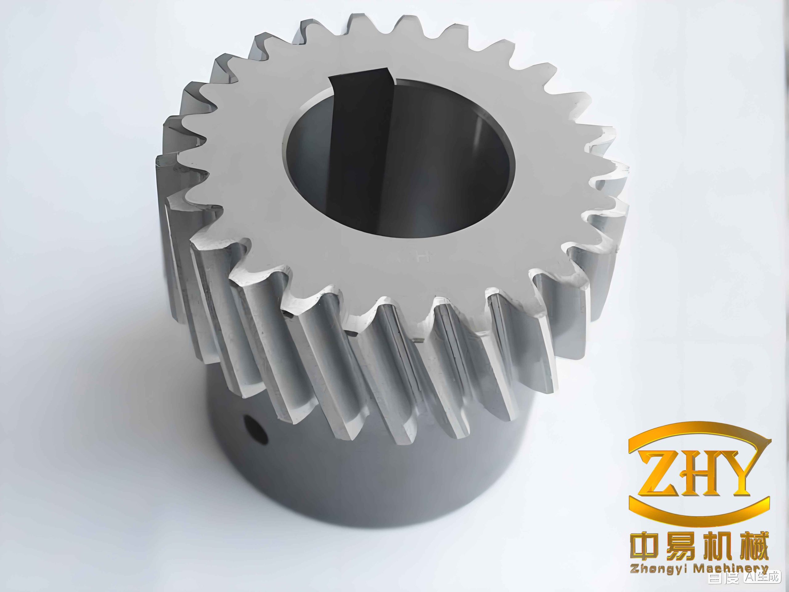
The main challenge for helical gears is not merely heating the surface, but obtaining a uniform temperature field along both the tooth profile and the tooth width. If the tooth tip overheats while the root remains too cold, the hardened layer becomes uneven. If the middle of the tooth width becomes much hotter than the two end faces, the final hardness distribution is inconsistent. I therefore designed a one-quarter tooth-width profiling induction coil, built a motion platform that controls both linear speed and angular speed, and developed a numerical method called the dynamic coordinate system method to represent the variable-speed spiral motion of helical gears. I used finite element analysis to couple the electromagnetic field, temperature field, and motion field, and I validated the simulation through experiments.
To make the analysis clear, I first summarize the main symbols used in my model. These symbols appear repeatedly in the electromagnetic field equations, heat transfer equations, motion equations, and result tables.
| Symbol | Meaning | Typical Unit |
|---|---|---|
| \(T\) | Temperature | °C |
| \(t\) | Time | s |
| \(\rho\) | Density or electrical resistivity depending on context | kg/m³ or Ω·m |
| \(c\) | Specific heat capacity | J/(kg·°C) |
| \(k\) | Thermal conductivity | W/(m·°C) |
| \(q_v\) | Volumetric Joule heat source | W/m³ |
| \(\mathbf{J}\) | Current density vector | A/m² |
| \(\mathbf{E}\) | Electric field intensity | V/m |
| \(\mathbf{B}\) | Magnetic flux density | T |
| \(\mathbf{H}\) | Magnetic field intensity | A/m |
| \(\mathbf{A}\) | Magnetic vector potential | Wb/m |
| \(\phi\) | Electric scalar potential | V |
| \(\sigma\) | Electrical conductivity | S/m |
| \(\mu\) | Magnetic permeability | H/m |
| \(\varepsilon\) | Permittivity | F/m |
| \(\delta\) | Current penetration depth | m |
| \(f\) | Current frequency | Hz |
| \(v_t\) | Instantaneous linear speed of helical gears | m/s |
| \(\omega_t\) | Instantaneous angular speed of helical gears | rad/s |
| \(r\) | Pitch radius | m |
| \(\beta\) | Helix angle | degree |
| \(s\) | Distance between adjacent heating positions | m |
| \(TH\) | Rotation angle of the local coordinate system | degree |
| \(\Delta T\) | Maximum temperature difference | °C |
The material chosen for the helical gears was 45 steel. Its chemical composition controls hardenability, strength, and response to induction heating. I used the nominal composition range to define the material model.
| Element | C | Si | Mn | Cr | Ni | Cu |
|---|---|---|---|---|---|---|
| Mass percentage (%) | 0.42–0.50 | 0.17–0.37 | 0.50–0.80 | 0.12–0.25 | 0.18–0.30 | 0.14–0.25 |
Because the electromagnetic and thermal properties of 45 steel change strongly with temperature, I treated them as nonlinear functions of temperature. I wrote discrete property data into a text file and let the finite element solver interpolate the values at each calculation step. This is important for helical gears because the skin depth, magnetic permeability, and heat generation rate all change rapidly near the Curie temperature.
| Temperature (°C) | Thermal conductivity \(k\) (W/(m·°C)) | Specific heat \(c\) (J/(kg·°C)) | Resistivity \(\rho\) (Ω·m) | Relative permeability \(\mu_r\) |
|---|---|---|---|---|
| 20 | 47.0 | 460 | 0.20×10⁻⁶ | 210 |
| 150 | 45.0 | 500 | 0.30×10⁻⁶ | 190 |
| 300 | 42.0 | 560 | 0.45×10⁻⁶ | 170 |
| 450 | 38.0 | 640 | 0.62×10⁻⁶ | 145 |
| 600 | 34.0 | 760 | 0.82×10⁻⁶ | 110 |
| 750 | 30.0 | 900 | 1.02×10⁻⁶ | 1 |
| 900 | 27.0 | 1000 | 1.14×10⁻⁶ | 1 |
| 1050 | 25.0 | 1050 | 1.20×10⁻⁶ | 1 |
I based the induction heating analysis on the fundamental electromagnetic induction law. When an alternating current flows through the induction coil, an alternating magnetic field is produced around the coil. This alternating field cuts the helical gears and induces an electromotive force. Because the helical gears form a closed conductive path, an eddy current is generated. The eddy current produces Joule heat in the surface layer. The induced electromotive force can be written as
$$E = -N\frac{d\Phi}{dt}$$
The induced current depends on the electromotive force and the impedance of the closed loop:
$$I = \frac{E}{Z} = \frac{E}{\sqrt{R^2+X^2}}$$
The Joule heat generated in the surface layer is expressed by
$$Q = 0.24 I^2 R t$$
For high-frequency induction heating of helical gears, the current penetration depth is a controlling parameter. I used the standard penetration depth formula:
$$\delta = 50300\sqrt{\frac{\rho}{\mu f}}$$
This equation shows that the penetration depth decreases as frequency increases and as permeability increases. When the temperature of the helical gears exceeds the Curie point, the relative permeability drops sharply to approximately unity, the skin depth increases, and the heat generation pattern changes. This behavior is essential for understanding the temperature curves of helical gears during high-frequency induction heating.
Several electromagnetic effects influence the temperature distribution in helical gears. I summarized their roles in the following table.
| Effect | Physical Meaning | Influence on Helical Gears |
|---|---|---|
| Skin effect | Alternating current concentrates near the surface | Heats the tooth surface and root layer quickly |
| Proximity effect | Magnetic fields of adjacent conductors interact | Requires constant coil-tooth gap for uniform heating |
| Ring effect | Current concentrates on the inner side of a ring-like coil | Improves energy utilization around the helical gears |
| Edge effect | Sharp corners attract higher eddy current density | Can overheat tooth tips of helical gears |
| End effect | Impedance changes near the workpiece ends | Causes temperature differences at the two end faces |
I modeled the electromagnetic field using Maxwell’s equations. In differential form, the equations are
$$\nabla \times \mathbf{H} = \mathbf{J}$$
$$\nabla \times \mathbf{E} = -\frac{\partial \mathbf{B}}{\partial t}$$
$$\nabla \cdot \mathbf{D} = 0$$
$$\nabla \cdot \mathbf{B} = 0$$
The constitutive relations are
$$\mathbf{D} = \varepsilon \mathbf{E}$$
$$\mathbf{J} = \sigma \mathbf{E}$$
$$\mathbf{B} = \mu \mathbf{H}$$
To solve the eddy current problem in helical gears, I introduced the magnetic vector potential \(\mathbf{A}\) and the electric scalar potential \(\phi\). The magnetic flux density and electric field can be expressed as
$$\mathbf{B} = \nabla \times \mathbf{A}$$
$$\mathbf{E} = -\frac{\partial \mathbf{A}}{\partial t} – \nabla \phi$$
The current density then becomes
$$\mathbf{J} = -\sigma \frac{\partial \mathbf{A}}{\partial t} – \sigma \nabla \phi$$
The coupled electromagnetic equations solved in the finite element model are
$$\nabla \times \left(\frac{1}{\mu}\nabla \times \mathbf{A}\right) + \sigma \frac{\partial \mathbf{A}}{\partial t} + \sigma \nabla \phi = 0$$
$$\nabla \cdot \left(-\sigma \frac{\partial \mathbf{A}}{\partial t} – \sigma \nabla \phi\right) = 0$$
For the temperature field, I treated the Joule heat generated by the eddy current as the internal heat source. The volumetric heat source is
$$q_v = \rho J^2$$
The transient heat conduction equation for helical gears is
$$\rho c \frac{\partial T}{\partial t} = \frac{\partial}{\partial x}\left(k\frac{\partial T}{\partial x}\right) + \frac{\partial}{\partial y}\left(k\frac{\partial T}{\partial y}\right) + \frac{\partial}{\partial z}\left(k\frac{\partial T}{\partial z}\right) + q_v$$
For the surfaces of the helical gears, I applied convection and radiation boundary conditions. A general boundary condition can be written as
$$-k\frac{\partial T}{\partial n} = h(T_w – T_f) + \epsilon \sigma_b (T_w^4 – T_0^4)$$
where \(h\) is the convection coefficient, \(T_w\) is the workpiece surface temperature, \(T_f\) is the ambient fluid temperature, \(\epsilon\) is the emissivity, and \(\sigma_b\) is the Stefan–Boltzmann constant. I also imposed an initial condition:
$$T(x,y,z,0) = T_0 = 25^\circ\text{C}$$
The design of the induction coil was critical for the heating quality of helical gears. I followed three main design rules. First, the copper tube wall thickness should exceed the hot penetration depth, and a value near \(1.57\delta\) provides a good compromise between electrical loss and mechanical strength. Second, the axial width of the copper tube determines the effective heating area and should be selected according to the maximum allowable current density. Third, the ratio of coil inner diameter to workpiece outer diameter should lie between approximately 1.1 and 2.0 to maintain reasonable heating efficiency while avoiding short circuits.
| Design Item | Selected Value or Rule | Reason |
|---|---|---|
| Coil material | Rectangular copper tube | High electrical conductivity and water cooling capability |
| Wall thickness | \(a = 1.57\delta\) | Above hot penetration depth, lower resistance |
| Axial width | \(b = I/(a\sigma_{\max})\) | Controls effective heating area and current capacity |
| Coil-to-tooth-tip gap | 6 mm | Reduces edge overheating and avoids contact |
| Coil-to-root gap | 3 mm | Improves root heating through proximity effect |
| Coil axial width | 10 mm | One-quarter of tooth width for layer-by-layer heating |
| Cooling method | Internal water flow | Prevents coil overheating and maintains stable impedance |
I initially considered a circular coil, a full profiling coil, and a “convex-shaped” profiling coil. The circular coil produced a magnetic field that was not perpendicular to the tooth surface, causing the tooth tip to overheat and the root to remain too cold. The full profiling coil improved the magnetic field orientation, but the magnetic flux concentrated in the middle of the coil, so the middle of the tooth width became hotter than the two end faces. The convex-shaped profiling coil reduced the middle overheating but required much higher power and lowered efficiency. I therefore selected a one-quarter tooth-width profiling coil for layer-by-layer heating of helical gears. This coil reduced manufacturing cost, simplified water cooling, and helped suppress the end effect along the tooth width.
I built the geometry of the helical gears and the one-quarter tooth-width profiling coil in a parametric solid modeler. The helical gears had a module of 4.5 mm, 12 teeth, a tooth width of 40 mm, and a helix angle of 10°. The coil was made from rectangular copper tube with a cross-section of 10 mm × 6 mm × 2 mm. The coil was manufactured by additive manufacturing because the profiling shape of the helical gears made conventional machining difficult.
| Parameter | Value | Parameter | Value |
|---|---|---|---|
| Module \(m\) | 4.5 mm | Coil-to-tip gap | 7.5 mm |
| Number of teeth \(z\) | 12 | Coil-to-root gap | 2.5 mm |
| Tooth width \(b\) | 40 mm | Coil cross-section \(S\) | 3252.5 mm² |
| Helix angle \(\beta\) | 10° | Coil axial width | 10 mm |
| Pitch diameter \(d\) | 64.4 mm | Current density \(J\) | 7.5×10⁷ A/m² |
| Initial temperature | 25 °C | Current frequency \(f\) | 100 kHz |
The motion of helical gears relative to the induction coil is a variable-speed spiral motion. The helical gears move downward along the axial direction while rotating around their own axis. The instantaneous linear speed \(v_t\) and instantaneous angular speed \(\omega_t\) must satisfy the relation
$$v_t = \omega_t r \tan\beta$$
Because \(r\) and \(\beta\) are fixed for a given helical gear, the linear speed and angular speed are proportional. I can therefore control the spiral motion by controlling either the linear speed or the angular speed. To represent this motion without rebuilding the entire mesh at every instant, I proposed the dynamic coordinate system method. In this method, the continuous motion of helical gears is equivalent to a sequence of static heating positions. At each position, I rotate a local coordinate system group by an angle \(TH\), apply the current density load, solve the electromagnetic and thermal fields, and then move to the next position.
The rotation angle of the local coordinate system between two adjacent heating positions is
$$TH = \frac{s \tan\beta}{r} \times \frac{180}{\pi}$$
where \(s\) is the distance between adjacent heating positions. If the total travel distance is \(d\), the number of heating positions is
$$k = \frac{d}{s}$$
I divided one tooth of the profiling coil into eight geometric segments. At the midpoints of the tooth tip, the two tooth flanks, and the root straight section, I created Cartesian local coordinate systems. At the center of the root arc, I created a cylindrical local coordinate system. I then rotated this set clockwise by \(360^\circ/z\) and repeated the procedure \(z-1\) times. This produced a complete local coordinate system group for one heating position. For a 12-tooth helical gear, the group contained 96 local coordinate systems: 48 Cartesian systems and 48 cylindrical systems.
I used the finite element method to solve the coupled electromagnetic-thermal-motion problem. The electromagnetic analysis was a harmonic eddy current analysis. The thermal analysis was a transient heat conduction analysis. I used a sequential coupling scheme. In each heating position, the electromagnetic solver calculated the eddy current and Joule heat. The Joule heat was then applied as an internal heat source in the thermal solver. The thermal solver calculated the temperature distribution, which became the initial temperature condition for the next electromagnetic solution. This process repeated until the induction coil passed through all heating positions along the tooth width.
| Region | Electromagnetic Element | Electromagnetic Material Properties | Thermal Element | Thermal Material Properties |
|---|---|---|---|---|
| Helical gears | SOLID117 | Relative permeability, resistivity | SOLID90 | Thermal conductivity, specific heat |
| Induction coil | SOLID117 | Relative permeability, resistivity | NULL | Not considered |
| Air | SOLID117 | Relative permeability | NULL | Not considered |
I created a cylindrical air domain with a volume about five times that of the helical gears. This domain fully enclosed the helical gears and the coil. The outer boundary of the air domain satisfied the magnetic flux normal condition, which was automatically handled by the finite element formulation. For the thermal analysis, I applied convection and radiation on the surfaces of the helical gears, while the coil and air temperatures were assumed constant because the coil had internal water cooling.
I wrote a parametric program in APDL to automate the simulation. The program first collected the gear geometry, helix angle, tooth width, and coil travel distance. It then built the local coordinate systems, imported the geometry groups, assigned materials and elements, generated the mesh, applied the current density load, solved the electromagnetic field, transferred the Joule heat to the thermal solver, and saved the nodal temperatures. After that, it rotated the local coordinate systems, imported the next geometry group, read the previous temperature results, and repeated the solution. This loop continued until all heating positions were completed.
The electromagnetic results showed that the magnetic flux density around the helical gears was strongly nonuniform. I defined three paths on the middle cross-section of the initial heating position: a path from one tooth tip center to the adjacent tooth tip center, a radial path from the tooth tip center to the gear center, and a path connecting the left and right tooth flank points on the pitch circle. Along the first path, the magnetic flux density decreased from the tooth tip to the root, but the middle of the root showed an increase because of the ring effect and proximity effect. Along the radial path, the magnetic flux density decayed exponentially from the surface to the core. Along the pitch-circle path, the magnetic flux density first decreased and then increased, and the left flank had a slightly higher maximum than the right flank because of the helix angle.
| Path | Location | Observed Magnetic Flux Density Trend |
|---|---|---|
| Tooth-tip to tooth-tip | Along the profile | High at the tooth tip, lower at the flank, local rise at the root middle |
| Tooth tip to center | Radial direction | Exponential decay from the surface to the core |
| Left flank to right flank | Pitch circle | First decreases, then increases; left side slightly higher |
I then analyzed the temperature field at the initial heating position. The temperature increase was fastest at the tooth tip because of the edge effect. The root heated quickly because it was closest to the coil and benefited from the proximity effect. The tooth flank heated more slowly at first. When the surface temperature exceeded the Curie point, the relative permeability dropped, the eddy current heat generation decreased, and the heating rate slowed. Heat then conducted from the tooth tip and root toward the flank and the core. Eventually, a relatively uniform temperature field formed along the tooth profile.
| Heating Time (s) | Tooth Tip Temperature (°C) | Flank Temperature (°C) | Root Temperature (°C) |
|---|---|---|---|
| 2.5 | 620 | 410 | 560 |
| 5.0 | 840 | 690 | 835 |
| 7.5 | 900 | 850 | 910 |
| 10.0 | 940 | 905 | 935 |
| 14.0 | 955 | 930 | 950 |
Along the tooth width, I divided the helical gear into four heating layers: d1, d2, d3, and d4. Each layer contained ten equally spaced heating positions. The coil moved from the lower end face to the upper end face. When the coil was in the first layer, the heat flux concentrated near the lower end face. As the coil moved to the middle layer, heat conduction from the lower layer combined with the newly generated Joule heat, so the heat flux became more evenly distributed along the tooth profile. This layer-by-layer strategy reduced the maximum temperature difference along the tooth width.
I compared two induction heating methods: overall heating and layer-by-layer heating. In overall heating, the coil width was equal to the full tooth width. In layer-by-layer heating, the coil width was one-quarter of the tooth width. The maximum temperature difference \(\Delta T\) was used as the quality index. A smaller \(\Delta T\) indicates a more uniform temperature field. I set a practical criterion that \(\Delta T \leq 50^\circ\text{C}\) is acceptable for uniform hardening of helical gears.
| Heating Method | Coil Width | Typical Temperature Trend | Maximum Temperature Difference | Assessment |
|---|---|---|---|---|
| Overall heating | Full tooth width | Middle higher, two end faces lower | About 87 °C | Less uniform |
| Layer-by-layer heating | One-quarter tooth width | More uniform along tooth width | About 18–42 °C depending on parameters | Better for helical gears |
I studied the effect of the initial and final heating positions. The initial position was defined by the distance \(L\) between the lower end face of the coil and the lower end face of the helical gears. I tested \(L = 0\) mm, \(L = 5\) mm, and \(L = 10\) mm. Increasing \(L\) gave the lower end face more preheating time and reduced the temperature difference between the middle and the ends. However, increasing \(L\) also increased the total heating time and reduced productivity. The best compromise among the tested values was \(L = 10\) mm.
| Initial Coil Distance \(L\) (mm) | Maximum Temperature Difference \(\Delta T\) (°C) | Observation |
|---|---|---|
| 0 | 70 | Large end-face temperature difference |
| 5 | 42 | Improved uniformity |
| 10 | 18 | Best uniformity among tested values |
I also studied the effect of coil moving speed. Two speed-loading modes were compared: a sudden-change mode and a gradual-change mode. In the sudden-change mode, the coil speed jumped from 1 mm/s to 2.5 mm/s. In the gradual-change mode, the speed increased from 1 mm/s to 2.5 mm/s in small increments of 0.15 mm/s per heating position. The gradual-change mode produced a smoother temperature curve and avoided sudden temperature drops. Therefore, the gradual-change mode was better for reducing internal stress and improving the uniformity of hardened layers in helical gears.
| Speed Loading Mode | Speed Change | Temperature Curve Feature | Maximum Temperature Difference |
|---|---|---|---|
| Sudden change | 1 mm/s to 2.5 mm/s instantaneously | Sudden temperature drop | Larger |
| Gradual change | 1 mm/s to 2.5 mm/s in steps | Smooth transition | Smaller |
I then varied the average coil moving speed from 1.5 mm/s to 2.5 mm/s and 3.5 mm/s. Lower speeds produced higher temperatures and faster heating, but they also increased the temperature difference between the middle and the ends. Higher speeds made the temperature distribution more uniform, but if the speed was too high, the heating time became insufficient and the middle of the tooth width could fail to reach the hardening temperature. Thus, the coil speed must be selected to balance uniformity and complete austenitization.
| Coil Speed (mm/s) | Maximum Temperature Difference \(\Delta T\) (°C) | Heating Quality Trend |
|---|---|---|
| 1.5 | 55 | Higher temperature, less uniform |
| 2.5 | 34 | More uniform |
| 3.5 | 22 | Most uniform, but risk of insufficient heating |
I also investigated the effect of current density. I tested \(6.0\times10^7\) A/m², \(7.5\times10^7\) A/m², and \(9.0\times10^7\) A/m². The current density directly controls the eddy current magnitude and the Joule heat. A moderate current density of \(7.5\times10^7\) A/m² produced the most uniform temperature along the tooth profile. When the current density was too high, the tooth tip became much hotter than the root and flank because of the edge effect and skin effect. When the current density was too low, the surface temperature might not reach the required hardening temperature.
| Current Density (A/m²) | Maximum Profile Temperature Difference \(\Delta T\) (°C) | Observation |
|---|---|---|
| 6.0×10⁷ | 45 | Lower heat input, risk of underheating |
| 7.5×10⁷ | 30 | Best uniformity in the tested range |
| 9.0×10⁷ | 58 | Overheating near the tooth tip |
The current frequency also affected the temperature distribution of helical gears. I tested 80 kHz, 100 kHz, and 120 kHz. Increasing the frequency intensified the skin effect and reduced the penetration depth. As a result, the surface heated faster while the deeper layer heated more slowly. The maximum temperature difference along the tooth profile increased with frequency. Therefore, a moderate reduction in frequency can reduce the temperature difference caused by the skin effect, but the frequency must still be high enough to achieve the required hardened layer depth.
| Current Frequency (kHz) | Maximum Profile Temperature Difference \(\Delta T\) (°C) | Observation |
|---|---|---|
| 80 | 28 | Lower skin effect, more uniform profile temperature |
| 100 | 34 | Balanced heating depth and uniformity |
| 120 | 49 | Stronger skin effect, larger profile difference |
After the numerical study, I performed high-frequency induction heating experiments on the helical gears. The experimental system included a high-frequency power supply, a water-cooling system, a one-quarter tooth-width profiling induction coil, a motion platform, and a temperature measurement system. The motion platform used a lead screw slide, a rotating motor, and a chuck to produce the variable-speed spiral motion of the helical gears. A programmable logic controller coordinated the linear and rotational motions. The temperature measurement system used K-type thermocouples and a data acquisition unit connected to a computer.
| Experimental Parameter | Value |
|---|---|
| Gear module | 4.5 mm |
| Number of teeth | 12 |
| Tooth width | 40 mm |
| Helix angle | 10° |
| Coil tube cross-section | 10 mm × 6 mm × 2 mm |
| Coil-to-tip gap | 6 mm |
| Coil-to-root gap | 3 mm |
| Current frequency | 100 kHz |
| Peak current | 3000 A |
| Current density | 7.5×10⁷ A/m² |
| Initial temperature | 25 °C |
| Cooling method | Water spray after heating |
The current density used in the simulation was calculated from the measured peak current and the effective cross-section of the copper tube near the helical gears:
$$J = \frac{I_{\max}}{S} = \frac{3000}{10\times2\times10^{-6}} = 7.5\times10^7\ \text{A/m}^2$$
I divided the tooth width into four layers and assigned different linear and angular speeds to each layer. The speed followed a slow-fast-fast-slow pattern to avoid local underheating. The linear speed and angular speed satisfied the spiral motion relation \(v_t = \omega_t r \tan\beta\).
| Heating Layer | Linear Speed (m/s) | Angular Speed (rad/s) | Heating Time (s) |
|---|---|---|---|
| d1 | 1.0×10⁻³ | 2.0×10⁻² | 10 |
| d2 | 2.5×10⁻³ | 5.1×10⁻² | 4 |
| d3 | 2.5×10⁻³ | 5.1×10⁻² | 4 |
| d4 | 1.0×10⁻³ | 2.0×10⁻² | 10 |
I installed four thermocouples on the helical gears. Point A was at the tooth tip center near the lower end face. Point B was at the intersection of the pitch circle and the right tooth flank near the lower end face. Point C was at the root center near the lower end face. Point D was at the intersection of the pitch circle and the right tooth flank at the middle of the tooth width. This arrangement allowed me to compare temperature evolution along both the tooth profile and the tooth width.
| Measurement Point | Location | Purpose |
|---|---|---|
| A | Tooth tip center, lower end region | Monitor edge-effect heating |
| B | Pitch circle and right flank, lower end region | Monitor flank heating |
| C | Root center, lower end region | Monitor root heating |
| D | Pitch circle and right flank, tooth-width middle | Monitor width-direction uniformity |
The experimental temperature curves showed the same general trend as the simulated curves. The temperature rose quickly below the Curie point, then slowed sharply after the material lost ferromagnetism. The tooth tip heated fastest, the root heated second fastest, and the flank heated more slowly at the beginning. Along the tooth width, the middle point D heated slightly faster than the lower-end point B because the end faces experienced a shorter effective heating time. By adjusting the initial position and the gradual speed profile, I reduced this difference.
| Measurement Point | Simulated Temperature at 20 s (°C) | Experimental Temperature at 20 s (°C) | Difference (°C) |
|---|---|---|---|
| A | 933.7 | 955.0 | 21.3 |
| B | 908.3 | 925.0 | 16.7 |
| C | 924.2 | 945.0 | 20.8 |
| D | 914.5 | 935.0 | 20.5 |
The experimental temperatures were slightly higher than the simulated temperatures. I attribute this difference to several factors. The actual thermal boundary conditions differed from the idealized simulation conditions. The thermocouples themselves were located in the alternating magnetic field and could develop small eddy currents, which slightly increased their measured temperature. The coil-to-workpiece gap may also have varied slightly during the experiment. Despite these effects, the maximum relative temperature error was about 3.1%, and the experimental and numerical curves agreed well. This validated the electromagnetic-thermal-motion coupling model and the dynamic coordinate system method for helical gears.
From the overall study, I conclude that layer-by-layer heating with a one-quarter tooth-width profiling coil is more suitable than overall heating for the helical gears considered here. The layer-by-layer method reduces the maximum temperature difference along the tooth width and lowers the power requirement. The start and end positions should be extended slightly beyond the tooth width to provide preheating and reduce end-face heat loss. The coil speed should use a gradual change rather than a sudden change. The current density and frequency should be selected together to balance hardened depth, temperature uniformity, and energy efficiency.
| Process Factor | Recommended Trend | Reason |
|---|---|---|
| Heating method | Layer-by-layer | Smaller width-direction temperature difference |
| Initial coil distance | About 10 mm | Provides preheating and reduces end effect |
| Speed loading | Gradual change | Avoids sudden temperature drops |
| Coil speed | Moderate, not too high | Balances uniformity and complete austenitization |
| Current density | Moderate | Reduces tip overheating and underheating risk |
| Current frequency | Moderate | Controls skin effect and hardened depth |
I also note several limitations that should be addressed in future work. I focused mainly on overall heating and layer-by-layer heating, but I did not perform a full orthogonal optimization of all geometric, motion, and electrical parameters together. I did not compare the layer-by-layer results with a complete set of results from circular coils and convex-shaped profiling coils under identical conditions. In addition, the simulation assumed constant coil and air temperatures, while in practice the coil impedance and cooling conditions may vary slightly. These factors can be included in future models to further improve the prediction accuracy for helical gears.
In summary, I developed a coupled numerical and experimental approach for high-frequency induction heating of helical gears used in heavy-duty truck transmissions. I designed a one-quarter tooth-width profiling induction coil, represented the variable-speed spiral motion through the dynamic coordinate system method, solved the electromagnetic-thermal-motion problem with sequential coupling, and validated the model through thermocouple experiments. The results show that uniform temperature distribution along both the tooth profile and tooth width of helical gears can be achieved by controlling the heating method, initial coil position, coil speed profile, current density, and current frequency. This work provides a quantitative basis for designing induction hardening processes for helical gears and for improving their load capacity, wear resistance, surface hardness, and service life.