
In this study, I focus on the coupled tribological and dynamic behavior of helical gears operating under finite line contact conditions. My aim is to explain how friction, time-varying meshing stiffness, dynamic mesh force, thermal elastohydrodynamic lubrication, and multi-directional gear vibration interact in a single coherent framework. Unlike a purely static lubrication analysis, I treat the contact load as a time-dependent quantity, and I also allow the lubricant shear stress to feed back into the dynamic equations through friction force and friction torque. This is important because helical gears frequently operate under high speed and high torque, where the oil film pressure, film thickness, temperature, and friction coefficient all fluctuate along the line of action. The resulting behavior cannot be captured accurately if the lubrication model uses only a constant nominal load or if the dynamic model ignores friction. Therefore, I develop single-degree-of-freedom and multi-degree-of-freedom dynamic models, one-way coupling models, and a fully coupled tribo-dynamic model for helical gears.
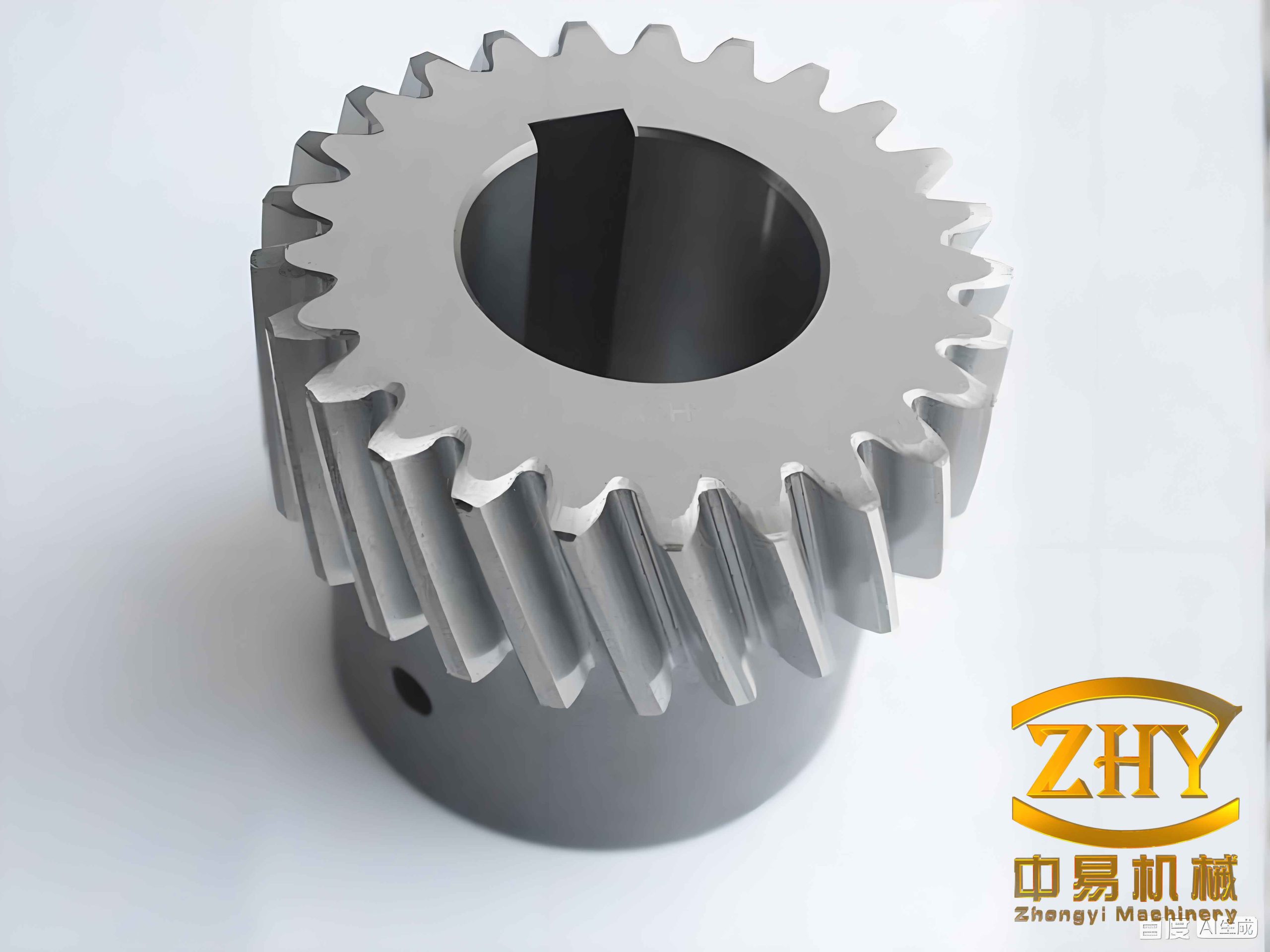
I begin from the observation that helical gears differ from spur gears because their contact line is inclined relative to the gear axis, and the contact line length changes continuously during meshing. This finite line contact behavior means that an infinitely long line contact assumption is not adequate. In my model, each meshing instant is represented by an equivalent contact between two opposed conical bodies, and the local curvature, entrainment velocity, sliding velocity, and slide-to-roll ratio are evaluated along the instantaneous contact line. I use these kinematic quantities in both the friction calculation and the thermal elastohydrodynamic lubrication calculation. The dynamic model supplies the instantaneous load and surface velocity, while the lubrication model supplies the shear stress, from which I compute the friction force and friction torque. This loop is repeated until the dynamic mesh force converges. By doing so, I can examine the coupling mechanism in helical gears rather than treating lubrication and dynamics as separate problems.
The following sections present the parametric excitations, the single-degree-of-freedom torsional model, the multi-degree-of-freedom coupled vibration model, the thermal elastohydrodynamic lubrication equations, the one-way coupling results, and the fully coupled tribo-dynamic results. I also include tables and equations to summarize the most important relationships. Throughout the article, I emphasize helical gears because their axial, transverse, torsional, and bending motions are coupled, and because their contact line geometry makes the lubrication problem inherently transient.
Parametric Excitations in Helical Gears
In my formulation, the main internal excitations of helical gears are the time-varying meshing stiffness, the transmission error, and the friction excitation. The time-varying meshing stiffness is obtained by an energy method. I consider Hertz contact energy, bending energy, shear energy, and axial compression energy. For a single tooth pair, the Hertz contact stiffness is expressed as
$$k_h=\frac{\pi E L}{4(1-\nu^2)}$$
where \(E\) is the equivalent elastic modulus, \(L\) is the contact length, and \(\nu\) is Poisson’s ratio. The bending, shear, and axial compression energies are written as
$$U_b=\int_0^d \frac{\left[F_b(d-x)-M\right]^2}{2EI_x}\,dx$$
$$U_s=\int_0^d \frac{1.2F_s^2}{2GA_x}\,dx$$
$$U_a=\int_0^d \frac{F_a^2}{2EA_x}\,dx$$
From these energies, I obtain the corresponding stiffness components \(k_b\), \(k_s\), and \(k_a\). The combined stiffness of one tooth pair is then
$$k_m(t)=\frac{1}{\frac{1}{k_h}+\frac{1}{k_{b1}}+\frac{1}{k_{s1}}+\frac{1}{k_{a1}}+\frac{1}{k_{b2}}+\frac{1}{k_{s2}}+\frac{1}{k_{a2}}}$$
When more than one tooth pair is in contact, I sum the contributions according to the contact ratio. In this way, the mesh stiffness of helical gears becomes a periodic function of meshing position. The static transmission error is represented as a periodic displacement excitation along the line of action:
$$e(t)=e_a\sin(\omega_e t+\phi_e)$$
where \(e_a\) is the error amplitude, \(\omega_e\) is the meshing frequency, and \(\phi_e\) is the phase angle. The friction excitation is obtained from the local friction coefficient and the local contact load along the instantaneous contact line. I calculate the local curvature radius, surface velocity, entrainment velocity, sliding velocity, and slide-to-roll ratio as functions of position and time.
For the finite line contact of helical gears, the local radii are expressed as
$$r_1(y,t)=r_{d1}(t)+y\sin\beta_b$$
$$r_2(y,t)=r_{d2}(t)-y\sin\beta_b$$
and the effective radii in the contact plane are
$$R_1(y,t)=r_1(y,t)\cos\beta_b$$
$$R_2(y,t)=r_2(y,t)\cos\beta_b$$
The equivalent radius is
$$R(y,t)=\frac{R_1(y,t)R_2(y,t)}{R_1(y,t)+R_2(y,t)}$$
The surface velocities of the two helical gears are
$$u_1(y,t)=\omega_1 r_1(y,t)\sin\beta_b$$
$$u_2(y,t)=\omega_2 r_2(y,t)\sin\beta_b$$
The entrainment velocity, sliding velocity, and slide-to-roll ratio are
$$u_e(y,t)=\frac{u_1(y,t)+u_2(y,t)}{2}$$
$$u_s(y,t)=u_1(y,t)-u_2(y,t)$$
$$\zeta(y,t)=\frac{u_s(y,t)}{u_e(y,t)}$$
These quantities vary along the contact line and also vary with meshing time. Because the contact line length of helical gears changes from the beginning to the end of engagement, the load per unit length is not uniform. I therefore discretize the contact line into small segments and compute the local friction force and friction torque. The friction coefficient is obtained from a generalized empirical relation that depends on the maximum Hertzian pressure, slide-to-roll ratio, entrainment velocity, equivalent radius, surface roughness, and lubricant viscosity. I express it in the general form
$$\mu=\exp\left[b_0+b_1\ln P_h+b_2\ln|SR|+b_3\ln V_e+b_4\ln\eta_0+b_5\ln R+b_6\ln S\right]$$
where \(P_h\) is the maximum Hertzian pressure, \(SR\) is the slide-to-roll ratio, \(V_e\) is the entrainment velocity, \(\eta_0\) is the ambient viscosity, \(R\) is the equivalent radius, and \(S\) is the composite surface roughness. The sign of the friction coefficient is determined by the direction of sliding. This relation allows me to obtain the friction coefficient quickly while still capturing the main lubrication effects in helical gears.
For a single tooth pair, the friction force at a discrete contact-line position is
$$f_k=\frac{1}{jj}\sum_{j=1}^{jj+1}\mu_{tj}F_{dk}L_t$$
where \(jj\) is the number of segments, \(\mu_{tj}\) is the local friction coefficient, \(F_{dk}\) is the dynamic load, and \(L_t\) is the local contact length. The total friction force includes the contribution of the reference tooth pair and the adjacent tooth pairs. The friction torque on the driving gear is
$$M_1=M_{pk}+M_{pak}+M_{pbk}$$
and the friction torque on the driven gear is
$$M_2=M_{gk}+M_{gak}+M_{gbk}$$
These friction torques enter the torsional dynamic equations. In helical gears, the friction force also enters the transverse vibration equation, which is one of the main reasons why friction cannot be neglected in a multi-degree-of-freedom model.
Single-Degree-of-Freedom Torsional Model of Helical Gears
I first establish a torsional dynamic model for a pair of helical gears. The model includes time-varying meshing stiffness, meshing damping, static transmission error, and friction torque. The equations of motion are
$$I_1\ddot{\theta}_1+c_m r_{b1}\dot{x}+k_m(t)r_{b1}x=T_1-M_1$$
$$I_2\ddot{\theta}_2-c_m r_{b2}\dot{x}-k_m(t)r_{b2}x=-T_2+M_2$$
where \(I_1\) and \(I_2\) are the rotary inertias, \(\theta_1\) and \(\theta_2\) are the angular displacements, \(r_{b1}\) and \(r_{b2}\) are the base radii, \(c_m\) is the meshing damping, \(k_m(t)\) is the time-varying meshing stiffness, \(T_1\) is the driving torque, \(T_2\) is the load torque, and \(M_1\) and \(M_2\) are the friction torques. The relative displacement along the line of action is defined as
$$x=r_{b1}\theta_1-r_{b2}\theta_2-e(t)$$
Using this relative displacement, I rewrite the torsional model as a single-degree-of-freedom equation:
$$m_e\ddot{x}+c_m\dot{x}+k_m(t)x=F_s+m_e\ddot{e}(t)+\frac{M_1}{r_{b1}}+\frac{M_2}{r_{b2}}$$
where \(m_e\) is the equivalent mass and \(F_s\) is the static mesh force. The dynamic mesh force is
$$F_d(t)=c_m\dot{x}+k_m(t)x$$
The dynamic transmission error, vibration velocity, vibration acceleration, and dynamic mesh force are solved by a variable-step Runge-Kutta method. I use the average mesh stiffness and the Hertzian half-width for non-dimensionalization. This improves numerical stability and allows me to compare different operating conditions. The dimensionless equation is
$$\ddot{X}+2\zeta \dot{X}+\bar{k}(\tau)X=\bar{F}_s+\ddot{\bar{e}}(\tau)+\bar{M}_1+\bar{M}_2$$
where \(X\) is the dimensionless relative displacement, \(\tau\) is the dimensionless time, \(\zeta\) is the damping ratio, \(\bar{k}(\tau)\) is the dimensionless mesh stiffness, and \(\bar{F}_s\) is the dimensionless static load. I find that friction has an edge effect on the dynamic response. When friction is included, the dynamic mesh force, dynamic transmission error, vibration velocity, and vibration acceleration deviate from the frictionless case, especially near the beginning and end of meshing. The effect is stronger when the friction coefficient is larger.
The gear parameters I use for the single-degree-of-freedom and multi-degree-of-freedom studies are summarized in the following table.
| Parameter | Value | Parameter | Value |
|---|---|---|---|
| Number of teeth of gear 1 | 28 | Number of teeth of gear 2 | 56 |
| Normal module | 7 mm | Pressure angle | 20 deg |
| Addendum coefficient | 1 | Clearance coefficient | 0.25 |
| Face width | 15 mm | Helix angle | 14 deg |
| Density of gear material | 7850 kg/m^3 | Equivalent elastic modulus | 227 GPa |
Multi-Degree-of-Freedom Tribo-Dynamic Model of Helical Gears
For a more realistic representation of helical gears, I establish an eight-degree-of-freedom model that includes transverse, axial, and torsional vibrations. The generalized coordinates are
$$\mathbf{X}=[y_1,y_2,x_1,x_2,z_1,z_2,\theta_1,\theta_2]^T$$
where \(y_i\) is the displacement along the line of action, \(x_i\) is the transverse displacement, \(z_i\) is the axial displacement, and \(\theta_i\) is the torsional displacement. The equations of motion are
$$m_1\ddot{y}_1+k_{y1}y_1+c_{y1}\dot{y}_1=-F_d\cos\beta$$
$$m_2\ddot{y}_2+k_{y2}y_2+c_{y2}\dot{y}_2=F_d\cos\beta$$
$$m_1\ddot{x}_1+k_{x1}x_1+c_{x1}\dot{x}_1=F_f$$
$$m_2\ddot{x}_2+k_{x2}x_2+c_{x2}\dot{x}_2=-F_f$$
$$m_1\ddot{z}_1+k_{z1}z_1+c_{z1}\dot{z}_1=-F_d\sin\beta$$
$$m_2\ddot{z}_2+k_{z2}z_2+c_{z2}\dot{z}_2=F_d\sin\beta$$
$$I_1\ddot{\theta}_1=T_1-F_d r_{b1}\cos\beta-M_1$$
$$I_2\ddot{\theta}_2=-T_2+F_d r_{b2}\cos\beta+M_2$$
Here \(F_f\) is the friction force, \(F_d\) is the dynamic mesh force, and \(\beta\) is the helix angle. The model can be written in matrix form as
$$[M]\ddot{\mathbf{X}}+[C]\dot{\mathbf{X}}+[K]\mathbf{X}=\mathbf{P}$$
where \([M]\), \([C]\), and \([K]\) are the mass, damping, and stiffness matrices, and \(\mathbf{P}\) is the excitation vector. The stiffness and damping matrices are symmetric. The excitation vector contains the dynamic mesh force components, friction force, friction torque, and transmission error terms.
The dynamic mesh force is obtained from the elastic deformation along the line of action:
$$\delta=(r_{b1}\theta_1-r_{b2}\theta_2)+(y_1-y_2)\cos\beta+(z_1-z_2)\sin\beta-e(t)$$
The normal dynamic mesh force is
$$F_d=k_m(t)\delta+c_m\dot{\delta}$$
The transverse and axial components are
$$F_{dy}=F_d\cos\beta$$
$$F_{dz}=F_d\sin\beta$$
The bearing support forces are
$$F_{byi}=k_{yi}y_i+c_{yi}\dot{y}_i$$
$$F_{bxi}=k_{xi}x_i+c_{xi}\dot{x}_i$$
$$F_{bzi}=k_{zi}z_i+c_{zi}\dot{z}_i$$
By solving the eigenvalue problem of the symmetric stiffness matrix with the average mesh stiffness, I obtain the natural frequencies and critical speeds of the helical gear system. The results are given in the following table.
| Mode | Natural frequency (Hz) | Critical speed (r/min) |
|---|---|---|
| 1 | 579.3 | 1241.4 |
| 2 | 515.6 | 1105.0 |
| 3 | 660.9 | 1416.0 |
| 4 | 1335.5 | 2862.0 |
| 5 | 1817.5 | 3894.7 |
| 6 | 2006.9 | 4300.4 |
| 7 | 2699.9 | 5785.4 |
The multi-degree-of-freedom model shows that the vibration in the direction of the line of action is the strongest. The axial and transverse vibrations are also significant because they are coupled with the torsional motion through the helix angle and friction. When I compare the single-degree-of-freedom and multi-degree-of-freedom results, I find that the multi-degree-of-freedom system can have several resonance regions, whereas the single-degree-of-freedom system has only one main resonance. At low speed, the dynamic load contains high-frequency components. At high speed, the dynamic load fluctuates strongly around the static load, and the amplitude depends on whether the operating speed is close to a natural frequency. Friction has a weak effect on pure torsional vibration, but it has a strong effect on transverse vibration. This occurs because the friction force acts in the transverse direction, and it can change the surface velocity of helical gears. Therefore, the surface velocity should be computed from the average kinematic velocity, the transverse vibration velocity, and the torsional vibration velocity.
Thermal Elastohydrodynamic Lubrication of Helical Gears
To capture the lubrication behavior of helical gears under dynamic load, I use a thermal elastohydrodynamic lubrication model based on finite line contact. The Reynolds equation is
$$\frac{\partial}{\partial x}\left(\frac{\rho h^3}{\eta}\frac{\partial p}{\partial x}\right)+\frac{\partial}{\partial y}\left(\frac{\rho h^3}{\eta}\frac{\partial p}{\partial y}\right)=12u_e\frac{\partial(\rho h)}{\partial x}+12\frac{\partial(\rho h)}{\partial t}$$
The film thickness equation is
$$h(x,y,t)=h_0(t)+h_g(x,y)+\frac{2}{\pi E’}\iint_\Omega \frac{p(x’,y’,t)}{\sqrt{(x-x’)^2+(y-y’)^2}}\,dx’dy’+s_1(x,y,t)+s_2(x,y,t)$$
where \(h_0\) is the rigid body displacement, \(h_g\) is the geometric gap, \(E’\) is the equivalent elastic modulus, and \(s_1\) and \(s_2\) are the surface roughness functions. For helical gears, the geometric gap includes both the transverse curvature and the end rounding. The load balance equation is
$$\iint_\Omega p(x,y,t)\,dxdy=F_w(t)$$
where \(F_w(t)\) is the load carried by one tooth pair. In the one-way coupling model, \(F_w(t)\) is the dynamic load from the multi-degree-of-freedom model. In the fully coupled model, \(F_w(t)\) is updated iteratively together with the friction force and friction torque.
I use a non-Newtonian lubricant model. The equivalent viscosity is
$$\eta^*=\frac{\eta}{\tau_0/\tau_e}\sinh\left(\frac{\tau_0}{\tau_e}\right)$$
The viscosity-pressure-temperature relation is
$$\eta=\eta_0\exp\left\{(\ln\eta_0+9.67)\left[(1+5.1\times10^{-9}p)^z-1\right]\right\}$$
and the density-pressure relation is
$$\rho=\rho_0\left[1+\frac{0.6\times10^{-9}p}{1+1.7\times10^{-9}p}\right]$$
The energy equation for the oil film is
$$\rho c_f\left(\frac{\partial T}{\partial t}+u_f\frac{\partial T}{\partial x}+v_f\frac{\partial T}{\partial y}\right)=\frac{\partial}{\partial z}\left(k_f\frac{\partial T}{\partial z}\right)+\eta\left[\left(\frac{\partial u_f}{\partial z}\right)^2+\left(\frac{\partial v_f}{\partial z}\right)^2\right]$$
The velocity components in the film are obtained from the Reynolds equation and the pressure gradient. The shear stress at the two surfaces is
$$\tau_1=\eta\frac{u_1-u_2}{h}+\frac{h}{2}\frac{\partial p}{\partial x}$$
$$\tau_2=\eta\frac{u_2-u_1}{h}-\frac{h}{2}\frac{\partial p}{\partial x}$$
The friction force is obtained by integrating the shear stress over the contact area:
$$F_f=\iint_\Omega (\tau_1+\tau_2)\,dxdy$$
The friction torque is
$$M_1=\iint_\Omega \tau_1 r_1(y,t)\,dxdy$$
$$M_2=\iint_\Omega \tau_2 r_2(y,t)\,dxdy$$
I solve the lubrication equations with a multigrid method or a direct iterative scheme. The elastic deformation is computed by a discrete Fourier transform algorithm, and the temperature field is solved by a column-by-column scanning method. The computational domain is discretized into \(128\times256\) nodes in the contact plane, with ten nodes across the film thickness and five nodes in each solid. The convergence tolerances are \(10^{-5}\) for pressure, \(10^{-4}\) for load, and \(10^{-5}\) for temperature. The lubricant and material parameters are listed in the following table.
| Parameter | Value |
|---|---|
| Ambient viscosity | 0.008 Pa s |
| Lubricant density | 870 kg/m^3 |
| Gear material density | 7850 kg/m^3 |
| Lubricant specific heat | 2000 J/(kg K) |
| Gear material specific heat | 470 J/(kg K) |
| Lubricant thermal conductivity | 0.14 W/(m K) |
| Gear material thermal conductivity | 46 W/(m K) |
| Pressure-viscosity coefficient | 2.2 GPa^-1 |
| Temperature-viscosity coefficient | 0.0476 K^-1 |
| Ambient temperature | 313 K |
| Characteristic shear stress | 5 MPa |
One-Way Coupling Between Dynamics and Lubrication
In the one-way coupling model, I first solve the multi-degree-of-freedom dynamic model for helical gears using an empirical friction coefficient. Then I use the resulting dynamic load as the load input to the thermal elastohydrodynamic lubrication model. This allows me to study how a time-varying load changes the oil film pressure, film thickness, temperature, and friction coefficient. I find that the dynamic load fluctuates around the static load. At very low speed, the dynamic load is close to the static load. As speed increases, the fluctuation amplitude becomes larger, and the dynamic load can even become negative in some intervals. The negative dynamic load indicates that the gear teeth may separate momentarily, which can cause impact and lubrication failure.
When the dynamic load is used in the lubrication model, the oil film pressure and film thickness fluctuate along the meshing line. The film thickness is strongly coupled to the pressure: where the dynamic load is high, the pressure is high and the film is thin; where the dynamic load is low, the pressure is low and the film is thick. This behavior is different from a static lubrication analysis, where the pressure and film thickness vary only because of the change in contact geometry and entrainment velocity. In helical gears, the finite line contact and the changing contact line length further complicate this behavior.
The temperature field is determined by both the dynamic load and the relative sliding velocity. Near the beginning and end of meshing, the sliding velocity is large, so the frictional heating is significant. In these regions, the oil film temperature is high. Near the pitch point, the sliding velocity is close to zero, so the temperature rise is very small. When the dynamic load is higher than the static load, the temperature rises; when the dynamic load is lower than the static load, the temperature falls. However, if the sliding velocity is very small, the load has only a weak effect on temperature. This is because the heat generation is proportional to the product of shear stress and sliding velocity. I also find that increasing speed increases the entrainment velocity and the film thickness, while the friction coefficient decreases. Increasing torque increases the dynamic load, increases the pressure, decreases the film thickness, increases the friction coefficient, and raises the temperature.
When surface roughness is included, the pressure, film thickness, and temperature fields show strong local fluctuations. At roughness peaks, the pressure can reach a local maximum, and stress concentration appears in the subsurface. At roughness valleys, the pressure drops, and the subsurface stress is lower. The locations of the pressure peaks correspond to the locations of the maximum subsurface stress. This is important for fatigue failure of helical gears, because the subsurface stress concentration can initiate cracks even when the nominal film thickness is adequate. The following table summarizes the main effects observed in the one-way coupling model.
| Condition | Pressure | Film thickness | Friction coefficient | Temperature |
|---|---|---|---|---|
| Speed increases | Fluctuates more | Increases | Decreases | Decreases |
| Torque increases | Increases | Decreases | Increases | Increases |
| Dynamic load high | Higher | Thinner | Higher | Higher if sliding is high |
| Pitch point | Moderate | Moderate | Near zero | Near ambient |
| Roughness peak | Local peak | Local minimum | Local rise | Local rise |
Fully Coupled Tribo-Dynamic Model of Helical Gears
The one-way coupling model assumes that the dynamic load is known before the lubrication calculation. In reality, the lubricant shear stress generates friction force and friction torque that change the gear vibration. Therefore, I establish a fully coupled tribo-dynamic model for helical gears. In this model, the dynamic equations and the thermal elastohydrodynamic lubrication equations are solved iteratively. The dynamic model provides the instantaneous dynamic load and surface velocity to the lubrication model. The lubrication model provides the shear stress, friction force, and friction torque to the dynamic model. The iteration continues until the dynamic load converges.
The surface velocity used in the lubrication model is not simply the kinematic velocity. It includes the effect of transverse vibration and torsional vibration:
$$u_1(y,t)=u_{1,kin}(y,t)+\dot{\theta}_1 r_1(y,t)-\dot{x}_1(t)$$
$$u_2(y,t)=u_{2,kin}(y,t)-\dot{\theta}_2 r_2(y,t)+\dot{x}_2(t)$$
where \(u_{1,kin}\) and \(u_{2,kin}\) are the nominal kinematic velocities, \(\dot{\theta}_1\) and \(\dot{\theta}_2\) are the torsional vibration velocities, and \(\dot{x}_1\) and \(\dot{x}_2\) are the transverse vibration velocities. The load carried by one tooth pair is
$$F_w(t)=\frac{L(t)}{L_z(t)}F_d(t)$$
where \(L(t)\) is the contact line length of one tooth pair and \(L_z(t)\) is the total contact line length. The convergence criterion is
$$e=\frac{\sum \left|F_w^{k+1}(t)-F_w^k(t)\right|}{\sum \left|F_w^{k+1}(t)\right|}<\varepsilon$$
where \(k\) is the iteration index and \(\varepsilon\) is the tolerance. I typically use \(\varepsilon=10^{-5}\). The iteration variables and their roles are summarized in the following table.
| Variable | From dynamics to lubrication | From lubrication to dynamics |
|---|---|---|
| Dynamic load | Load balance | Not applied |
| Surface velocity | Reynolds equation and energy equation | Not applied |
| Shear stress | Not applied | Friction force and torque |
| Friction coefficient | Not applied | Indirect through shear stress |
| Transverse vibration | Surface velocity update | Friction excitation |
| Torsional vibration | Surface velocity update | Friction torque |
I find that friction force and friction torque decrease as speed increases. This is because the film thickness increases with speed, and the lubricant shear stress decreases. At low speed, the film is thin, the shear stress is high, and the friction force and friction torque are large. Therefore, friction has a strong effect on the dynamic load at low speed. As speed increases, the friction effect becomes weaker. When the torque is increased, the friction force and friction torque increase, but their relative effect on the dynamic load depends on the operating speed. At very low torque, the friction effect on the dynamic load is small because the contact load itself is small.
In the fully coupled model, the oil film pressure and film thickness are different from the static case. At low speed, the center oil film pressure and average film thickness show high-frequency fluctuations. These fluctuations come from the time-varying dynamic load and the high-frequency components of the vibration. As speed increases, the high-frequency fluctuations disappear, and the pressure becomes smoother. However, the dynamic load is still time-varying, so the pressure and film thickness still differ from the static solution. The average film thickness in the coupled model can be larger or smaller than the static value depending on the operating condition. When the dynamic load is lower than the static load, the film is thicker; when the dynamic load is higher than the static load, the film is thinner.
The temperature field in the fully coupled model is also affected by the transverse vibration and torsional vibration. Because friction and friction torque change the surface velocity, the entrainment velocity and sliding velocity vary with time. This changes the frictional heating. At positions where the slide-to-roll ratio is high, the temperature is high. At positions where the slide-to-roll ratio is low, the temperature is low. In the static model, the center oil film temperature near the pitch point is almost equal to the ambient temperature. In the coupled model, the center oil film temperature can show additional peaks because the dynamic surface velocity changes the local sliding conditions. The friction coefficient in the coupled model is generally smaller than in the static model. This is because the coupled surface velocity is higher and the film thickness is larger. The reduction is more pronounced at low speed and high load.
The following table compares the static lubrication model and the fully coupled tribo-dynamic model for helical gears.
| Feature | Static lubrication model | Fully coupled tribo-dynamic model |
|---|---|---|
| Contact load | Constant nominal load | Time-varying dynamic load |
| Surface velocity | Kinematic only | Kinematic plus transverse and torsional vibration |
| Friction force | Not fed back | Fed back into dynamic equations |
| Friction torque | Not fed back | Fed back into torsional equations |
| Pressure fluctuation | Geometric only | Geometric plus dynamic |
| Film thickness fluctuation | Geometric only | Geometric plus dynamic |
| Temperature | Determined by nominal sliding | Determined by instantaneous sliding and load |
| Friction coefficient | Static estimate | Instantaneous coupled estimate |
Numerical Procedure and Stability
I solve the dynamic equations with a variable-step Runge-Kutta method. The equations are non-dimensionalized using the average mesh stiffness and the Hertzian half-width. This reduces numerical stiffness and improves convergence. The lubrication equations are solved on a fine grid. The elastic deformation is computed by a discrete Fourier transform algorithm, and the temperature field is solved by a column-by-column scanning method. The pressure and temperature loops are solved iteratively. The load balance is checked at every iteration. The convergence tolerances are set to \(10^{-5}\) for pressure, \(10^{-4}\) for load, and \(10^{-5}\) for temperature. In the fully coupled model, the dynamic load convergence tolerance is \(10^{-5}\). I find that at least fifty revolutions of the driving gear are required to reach a stable periodic solution. In my calculations, I use one hundred and twenty-eight revolutions and five hundred and twelve mesh points per tooth. This ensures that the dynamic response is fully developed and that the frequency content is accurately captured.
The numerical procedure can be summarized as follows. First, I set the friction force and friction torque to zero and solve the dynamic equations. Second, I use the resulting dynamic load and surface velocity in the thermal elastohydrodynamic lubrication model. Third, I compute the shear stress, friction force, and friction torque from the lubrication solution. Fourth, I insert the friction force and friction torque into the dynamic equations and solve again. Fifth, I repeat the process until the dynamic load converges. This procedure captures the two-way coupling between the dynamics and lubrication of helical gears.
Effects of Speed and Torque on Helical Gears
Speed has a strong effect on both the dynamics and lubrication of helical gears. In the dynamic model, increasing speed increases the dynamic load fluctuation. When the operating speed approaches a natural frequency, resonance occurs, and the dynamic load can be several times larger than the static load. In the multi-degree-of-freedom model, several resonance regions can appear because the transverse, axial, and torsional modes are coupled. This is different from the single-degree-of-freedom model, which has only one main resonance. In the lubrication model, increasing speed increases the entrainment velocity, which increases the film thickness. The friction coefficient decreases with speed because the film thickness increases and the shear rate decreases. The temperature also decreases with speed because the friction coefficient and shear stress decrease, even though the sliding velocity increases. This is a subtle result: at low speed, the film is thin, the shear stress is high, and the temperature can be high; at high speed, the film is thicker, the shear stress is lower, and the temperature can be lower.
Torque has the opposite effect. Increasing torque increases the dynamic load, which increases the oil film pressure and decreases the film thickness. The friction coefficient increases because the pressure is higher and the film is thinner. The temperature increases because the shear stress and frictional heating increase. In the dynamic model, increasing torque increases the static load and the dynamic load. The vibration amplitude also increases because the excitation force is larger. However, the relative effect of friction on the dynamic load is smaller at high torque because the contact load is already large. At low torque, the friction effect is also small because the contact load is small. The strongest friction effect on the dynamic load occurs at low speed and moderate torque.
The following table summarizes the combined effects of speed and torque on helical gears.
| Operating condition | Dynamic load | Film thickness | Friction coefficient | Temperature | Friction effect on dynamics |
|---|---|---|---|---|---|
| Low speed, low torque | Close to static | Thin | High | Low to moderate | Moderate |
| Low speed, high torque | High | Thin | High | High | Strong |
| High speed, low torque | Fluctuating | Thick | Low | Low | Weak |
| High speed, high torque | Strongly fluctuating | Moderate | Moderate | Moderate to high | Moderate |
Surface Roughness and Subsurface Stress in Helical Gears
Surface roughness plays an important role in the lubrication and fatigue of helical gears. When I include a two-dimensional sinusoidal roughness in the lubrication model, the oil film pressure, film thickness, and temperature fields become highly non-uniform. At roughness peaks, the film thickness is locally reduced, and the pressure rises sharply. This pressure peak creates a subsurface stress concentration. At roughness valleys, the film thickness is locally increased, and the pressure drops. The subsurface stress is lower at these locations. I find that the locations of maximum subsurface stress coincide with the locations of maximum oil film pressure. This means that roughness peaks are potential initiation sites for micropitting and fatigue cracks in helical gears.
The roughness effect is more pronounced when the film thickness is small. At low speed or high torque, the film is thin, and the roughness peaks can penetrate the film and contact the opposing surface. This leads to mixed lubrication, where the load is shared between the fluid film and the asperity contacts. In mixed lubrication, the friction coefficient is higher, and the temperature rise is larger. At high speed, the film is thicker, and the roughness effect is reduced. However, even in full-film lubrication, roughness can still cause local pressure fluctuations and subsurface stress concentrations. Therefore, surface roughness should be included in any comprehensive tribo-dynamic analysis of helical gears.
Summary of Key Findings
I have developed a series of models for helical gears, starting from a single-degree-of-freedom torsional model and progressing to a fully coupled tribo-dynamic model. The main findings are as follows. First, friction has a weak effect on pure torsional vibration but a strong effect on transverse vibration. In helical gears, the transverse vibration changes the surface velocity, which in turn changes the lubrication condition. Second, the dynamic load in helical gears is time-varying and can deviate significantly from the static load. At low speed, the dynamic load is close to the static load but contains high-frequency components. At high speed, the dynamic load fluctuates strongly and can cause resonance. Third, the oil film pressure and film thickness fluctuate with the dynamic load. In the one-way coupling model, the pressure and film thickness follow the dynamic load directly. In the fully coupled model, the friction force and friction torque feed back into the dynamic equations, which further modifies the dynamic load and surface velocity. Fourth, the temperature field is controlled by both the dynamic load and the sliding velocity. Near the pitch point, the temperature rise is small because the sliding velocity is small. Near the beginning and end of meshing, the temperature rise is large because the sliding velocity is large. Fifth, surface roughness creates local pressure peaks and subsurface stress concentrations. These stress concentrations are important for fatigue life prediction of helical gears.
Conclusions and Outlook
In this study, I established single-degree-of-freedom and multi-degree-of-freedom dynamic models for helical gears, a one-way coupling model between dynamics and thermal elastohydrodynamic lubrication, and a fully coupled tribo-dynamic model. The models include time-varying meshing stiffness, meshing damping, static transmission error, friction force, friction torque, transverse vibration, axial vibration, and torsional vibration. I solved the dynamic equations with a variable-step Runge-Kutta method and the lubrication equations with a thermal elastohydrodynamic lubrication solver. The results show that the coupling between friction and dynamics is significant, especially at low speed and high torque. The friction force and friction torque change the transverse and torsional vibrations, which change the surface velocity and the lubrication condition. The lubrication condition, in turn, changes the friction force and friction torque. This two-way coupling cannot be ignored in accurate predictions of the dynamic load, oil film pressure, film thickness, temperature, and friction coefficient of helical gears.
For future work, I plan to extend the model to helical gears with tooth defects, such as pitting, spalling, and cracks. These defects change the contact stiffness, contact line length, and lubrication condition, and they may cause local stress concentrations and temperature rises. I also plan to use the coupled model to predict fatigue life and to study the effect of profile modification on the tribo-dynamic behavior of helical gears. In addition, I intend to include the effect of bearing dynamics and housing flexibility in the multi-degree-of-freedom model, because these components can influence the vibration modes and the dynamic load of helical gears. Finally, I plan to validate the fully coupled model with more extensive experiments under different speeds, torques, lubricants, and surface roughness conditions.
Overall, my results demonstrate that helical gears should be analyzed as coupled tribo-dynamic systems. The interaction between friction, vibration, and thermal elastohydrodynamic lubrication determines the load capacity, efficiency, noise, and fatigue life of helical gears. By combining dynamic equations with thermal elastohydrodynamic lubrication equations in a fully coupled framework, I can capture the instantaneous behavior of helical gears more accurately than with static or uncoupled models. This approach provides a useful foundation for the design and analysis of high-performance helical gears in modern mechanical transmission systems.