
I propose a digital-model hybrid-driven fault diagnosis framework for wind turbine planetary gearboxes, with particular attention to the pinion gear as a critical rotating component. In my view, the central difficulty is not simply that wind turbine planetary gearboxes are complex mechanical systems. The deeper difficulty is that a pinion gear may remain healthy for long periods, while severe pinion gear faults such as tooth missing, tooth breakage, and root crack appear only rarely. Consequently, real measured fault samples are scarce, highly imbalanced, and expensive to collect. I combine a high-fidelity lumped-parameter dynamic model with a domain-shared residual network, local maximum mean discrepancy alignment, and a Kolmogorov-Arnold network classifier. The dynamic model generates pseudo-fault data for the pinion gear, and the deep model learns transferable physical features from both pseudo and measured signals. I validate the framework on two wind turbine planetary gearbox experimental settings under multiple speed conditions. The results show that my method maintains strong diagnostic accuracy when fault samples are scarce, and it outperforms several classical data-level, algorithm-level, and hybrid baselines.
Notation and core diagnostic quantities. I use the following notation to keep the derivation consistent. The pinion gear is treated as a central fault-sensitive component. The sun gear, ring gear, carrier, and planetary pinion gear are coupled through time-varying meshing stiffness. The mesh frequency, fault characteristic frequency, and speed relations are summarized in Table 1 and Eq. (1) through Eq. (4).
| Symbol | Meaning | Typical unit |
|---|---|---|
| \(z_s\) | Number of sun gear teeth | dimensionless |
| \(z_r\) | Number of ring gear teeth | dimensionless |
| \(z_p\) | Number of pinion gear teeth | dimensionless |
| \(n\) | Input shaft speed | r/min |
| \(f_s\) | Sun gear rotational frequency | Hz |
| \(f_m\) | Gear mesh frequency | Hz |
| \(f_{st}\) | Local fault characteristic frequency of the sun or pinion gear | Hz |
| \(m_l\) | Mass of component \(l\) | kg |
| \(k_l\) | Support stiffness of component \(l\) | N/m |
| \(c_l\) | Support damping of component \(l\) | N\(\cdot\)s/m |
| \(J_l\) | Rotational inertia of component \(l\) | kg\(\cdot\)m\(^2\) |
| \(r_l\) | Base circle radius of component \(l\) | mm |
| \(F\) | Dynamic meshing force | N |
| \(T_i, T_o\) | Input torque and output load torque | N\(\cdot\)m |
| \(\alpha\) | Pressure angle | degree |
| \(\psi_n\) | Angular position of the \(n\)-th pinion gear | rad |
The kinematic relations I use for the pinion gear system are:
$$
f_s = \frac{n}{60}
$$
$$
f_m = \frac{z_s z_r}{60(z_s+z_r)} n
$$
$$
f_{st} = \frac{f_m}{z_s}
$$
$$
\psi_n = \frac{2\pi(n-1)}{N_p}, \quad n=1,2,\ldots,N_p
$$
Here \(N_p\) is the number of planetary pinion gear branches. For a fixed-ring planetary gearbox, the carrier speed and the relative speed of each pinion gear determine the modulation sidebands around the mesh frequency. When a local pinion gear fault occurs, the time-varying meshing stiffness is perturbed periodically, and the resulting vibration response contains impulse components and modulation sidebands. These sidebands are the physical foundation of my pseudo-fault data generation.
Why I use a dynamic model for the pinion gear. A purely data-driven model requires a large amount of balanced fault data to learn a reliable decision boundary. In wind turbine planetary gearboxes, the healthy state dominates the operating history. A pinion gear fault often triggers shutdown or maintenance before a long fault record can be accumulated. I therefore use a physics-based dynamic model to synthesize fault responses for the pinion gear and use those responses as an auxiliary source domain. The dynamic model is not intended to replace measured data. Instead, it supplies physically meaningful fault patterns that guide feature learning when measured fault samples are few.
Lumped-parameter dynamic model. I adopt a lumped-parameter formulation because it is computationally efficient and can represent the dominant vibrations of the planetary gearbox, including the pinion gear meshing behavior. Each component has two translational degrees of freedom and one rotational degree of freedom. The sun gear, carrier, ring gear, and each pinion gear are connected by equivalent spring-damper elements. The equations of motion for the sun gear are:
$$
\begin{aligned}
m_s\left(\ddot{x}_s – x_s\omega_c^2 – 2\dot{y}_s\omega_c – y_s\dot{\omega}_c\right) + k_s x_s + c_s\dot{x}_s + \sum_{n=1}^{N_p} F_{spn}\cos\psi_{sn} &= 0,\\
m_s\left(\ddot{y}_s – y_s\omega_c^2 + 2\dot{x}_s\omega_c + x_s\dot{\omega}_c\right) + k_s y_s + c_s\dot{y}_s + \sum_{n=1}^{N_p} F_{spn}\sin\psi_{sn} &= 0,\\
\frac{J_s}{r_s}\ddot{\theta}_s + \sum_{n=1}^{N_p} F_{spn} &= \frac{T_i}{r_s}.
\end{aligned}
$$
The equations of motion for the carrier are:
$$
\begin{aligned}
m_c\left(\ddot{x}_c – x_c\omega_c^2 – 2\dot{y}_c\omega_c – y_c\dot{\omega}_c\right) + k_{cx}x_c + c_c\dot{x}_c – \sum_{n=1}^{N_p} F_{cpxn} &= 0,\\
m_c\left(\ddot{y}_c – y_c\omega_c^2 + 2\dot{x}_c\omega_c + x_c\dot{\omega}_c\right) + k_{cy}y_c + c_c\dot{y}_c – \sum_{n=1}^{N_p} F_{cpyn} &= 0,\\
\frac{J_c}{r_c}\ddot{\theta}_c + \sum_{n=1}^{N_p} F_{cpxn}\sin\psi_n – \sum_{n=1}^{N_p} F_{cpyn}\cos\psi_n &= \frac{T_o}{r_c}.
\end{aligned}
$$
The equations of motion for the ring gear are:
$$
\begin{aligned}
m_r\left(\ddot{x}_r – x_r\omega_c^2 – 2\dot{y}_r\omega_c – y_r\dot{\omega}_c\right) + c_r\dot{x}_r + k_r x_r + \sum_{n=1}^{N_p} F_{rpn}\cos\psi_{rpn} &= 0,\\
m_r\left(\ddot{y}_r – y_r\omega_c^2 + 2\dot{x}_r\omega_c + x_r\dot{\omega}_c\right) + c_r\dot{y}_r + k_r y_r + \sum_{n=1}^{N_p} F_{rpn}\sin\psi_{rpn} &= 0,\\
J_r\ddot{\theta}_r + c_{rt}\dot{\theta}_r + k_{rt}\theta_r + r_r\sum_{n=1}^{N_p} F_{rpn} &= 0.
\end{aligned}
$$
The equations of motion for each pinion gear are:
$$
\begin{aligned}
m_{pn}\left(\ddot{x}_{pn} – x_{pn}\omega_c^2 – 2\dot{y}_{pn}\omega_c – y_{pn}\dot{\omega}_c\right) + F_{cpxn} – (F_{spn}-F_{rpn})\cos\alpha &= 0,\\
m_{pn}\left(\ddot{y}_{pn} – y_{pn}\omega_c^2 + 2\dot{x}_{pn}\omega_c + x_{pn}\dot{\omega}_c\right) + F_{cpyn} – (F_{spn}+F_{rpn})\sin\alpha &= 0,\\
\frac{J_{pn}}{r_p}\ddot{\theta}_{pn} + F_{spn} – F_{rpn} &= 0.
\end{aligned}
$$
I solve these second-order nonlinear differential equations with a fourth-order variable-step Runge-Kutta method. The dynamic meshing forces couple the sun gear, ring gear, carrier, and every pinion gear. The stiffness of each mesh is time-varying, and the fault state of the pinion gear directly changes the mesh stiffness. Therefore, the dynamic model can generate distinct responses for a healthy pinion gear, a missing-tooth pinion gear, a broken-tooth pinion gear, and a cracked pinion gear.
Time-varying meshing stiffness. I calculate the time-varying meshing stiffness using the potential energy method. The total mesh stiffness includes Hertzian contact stiffness, bending stiffness, axial compression stiffness, shear stiffness, and foundation flexibility stiffness. The combined stiffness for one gear pair is:
$$
k = \sum_{i=1}^{2}\left(\frac{1}{k_h}+\frac{1}{k_{b1,i}}+\frac{1}{k_{s1,i}}+\frac{1}{k_{a1,i}}+\frac{1}{k_{f1,i}}+\frac{1}{k_{b2,i}}+\frac{1}{k_{s2,i}}+\frac{1}{k_{a2,i}}+\frac{1}{k_{f2,i}}\right)^{-1}.
$$
For external meshing, the two bodies in Eq. (8) are the sun gear and the pinion gear. For internal meshing, the two bodies are the pinion gear and the ring gear. I define the fault state by modifying the geometric and stiffness contributions of the pinion gear. A missing tooth removes one contact pair and produces a single-pair meshing interval. A broken tooth changes the contact area and creates a local stiffness drop. A root crack reduces the effective bending and shear stiffness, and the crack depth and angle control the severity of the stiffness reduction. These changes are propagated into the equations of motion, and the model outputs the corresponding time-domain and frequency-domain responses.
Model validation and pseudo-data characteristics. I compare pseudo signals with measured signals to ensure that the dynamic model captures the essential pinion gear fault signatures. The comparison focuses on time-domain impulse amplitude, mesh frequency location, and sideband structure. Table 2 summarizes a representative validation for a missing-tooth pinion gear fault. The pseudo signal and the measured signal are not identical, which is expected because the model simplifies damping, friction, and boundary conditions. However, the key physical features are consistent.
| Feature | Pseudo pinion gear signal | Measured pinion gear signal | Physical interpretation |
|---|---|---|---|
| Peak acceleration | Approximately 2.0 m/s\(^2\) | Approximately 1.1 m/s\(^2\) | Same order of magnitude and impulse-like |
| Mesh frequency | 106 Hz | 107.99 Hz | Close to theoretical mesh frequency |
| Dominant components | \(f_m, 2f_m, 3f_m,\ldots\) | \(f_m, 2f_m, 3f_m,\ldots\) | Mesh harmonics dominate both signals |
| Sidebands | Visible around mesh harmonics | Visible around mesh harmonics | Fault-induced amplitude modulation |
| Impulse periodicity | Related to pinion gear rotation | Related to pinion gear rotation | Local fault repeats once per revolution |
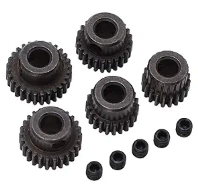
The validation confirms that the dynamic model generates physically plausible pseudo-fault data for the pinion gear. I use these pseudo signals to supplement the scarce measured fault samples. The source domain contains pseudo pinion gear data with abundant fault labels. The target domain contains measured healthy data and a small number of measured pinion gear fault samples. My goal is to learn a feature representation that aligns the two domains at the fault-category level while preserving discriminative fault information.
Domain-shared residual feature extractor. I design a domain-shared residual network as the feature extractor. The network is shared between the pseudo source domain and the measured target domain. I use a residual learning formulation because it stabilizes deep feature extraction and mitigates gradient degradation. A residual block can be written as:
$$
y = F(x, W) + x,
$$
where \(x\) is the input feature map, \(F(x,W)\) is the residual mapping, and \(y\) is the output. I further embed a convolutional block attention module into each residual block. The channel attention is:
$$
M_c(F) = \sigma\left(MLP(AvgPool(F)) + MLP(MaxPool(F))\right),
$$
and the spatial attention is:
$$
M_s(F) = \sigma\left(f^{7\times7}\left([AvgPool(F); MaxPool(F)]\right)\right).
$$
The final attention-refined feature is:
$$
F’ = M_s(M_c(F) \otimes F) \otimes (M_c(F) \otimes F).
$$
This attention mechanism helps the network focus on fault-sensitive regions and frequency components in the pinion gear vibration signal. In my experiments, the attention-refined residual features are more stable across speed conditions than plain convolutional features. The feature extractor is shared by the source and target domains, so the learned representation is not biased toward either pseudo data or measured data.
Local maximum mean discrepancy. To reduce the distribution gap between pseudo pinion gear data and measured pinion gear data, I introduce local maximum mean discrepancy. The global maximum mean discrepancy aligns marginal distributions, but it ignores class-specific structures. In a fault diagnosis problem, aligning the marginal distribution alone can mix different fault classes. I therefore align the conditional distributions of each fault category. The Gaussian kernel matrix is:
$$
K(X_s,X_t) = -\exp\left(-\frac{\|X_s-X_t\|^2}{2\sigma^2}\right).
$$
For each fault class \(c\), I compute instance weights from the one-hot label vector and the predicted distribution:
$$
W_i^c = \frac{p_i^c}{\sum_{i=1}^{N}p_i^c}.
$$
The local maximum mean discrepancy loss is:
$$
\begin{aligned}
L_{LMMD} &= \frac{1}{C}\sum_{c=1}^{C}\left\|\sum_{i=1}^{N_s}W_i^{sc}\phi(F_i^s)-\sum_{j=1}^{N_t}W_j^{tc}\phi(F_j^t)\right\|_H^2\\
&= \frac{1}{C}\sum_{c=1}^{C}\left[
\sum_{i=1}^{N_s}\sum_{j=1}^{N_s}W_i^{sc}W_j^{sc}K(F_i^s,F_j^s)
+\sum_{i=1}^{N_t}\sum_{j=1}^{N_t}W_i^{tc}W_j^{tc}K(F_i^t,F_j^t)
-2\sum_{i=1}^{N_s}\sum_{j=1}^{N_t}W_i^{sc}W_j^{tc}K(F_i^s,F_j^t)
\right].
\end{aligned}
$$
Here \(C\) is the number of fault categories, \(N_s\) is the number of source samples, \(N_t\) is the number of target samples, and \(\phi(\cdot)\) is the feature mapping. I minimize \(L_{LMMD}\) so that the same pinion gear fault class from the pseudo domain and the measured domain occupies a similar region in the latent feature space. This is especially important for pinion gear crack and pinion gear breakage, because these two faults can produce similar low-frequency modulation patterns if only global alignment is used.
Kolmogorov-Arnold network classifier. I use a Kolmogorov-Arnold network as the classifier. Unlike a standard multilayer perceptron that applies fixed activation functions at nodes, the Kolmogorov-Arnold network applies learnable activation functions on edges. Each activation is represented as a combination of a basis function and a spline function:
$$
\phi(x) = w_b b(x) + w_s \operatorname{spline}(x),
$$
where \(b(x)\) is a smooth basis function, and the spline is a linear combination of B-splines:
$$
\operatorname{spline}(x) = \sum_{i} c_i B_i(x).
$$
The B-spline activation provides smooth interpolation and noise suppression. In a wind turbine planetary gearbox, the measured pinion gear signal contains not only fault impulses but also electromagnetic interference, structural resonances, and random load fluctuations. The smooth spline representation helps the classifier avoid overfitting to high-frequency noise. The Kolmogorov-Arnold network also improves the modeling of complex nonlinear relations between latent features and fault labels. I use it as the final classification module after the domain-shared residual feature extractor.
Overall objective. The total loss combines classification loss, local maximum mean discrepancy loss, and regularization:
$$
L = L_{cls} + \lambda L_{LMMD} + \mu \|W\|_2^2,
$$
where \(L_{cls}\) is the cross-entropy loss over the fault categories, \(\lambda\) controls the domain alignment strength, and \(\mu\) controls weight decay. I optimize the network parameters by backpropagation. The feature extractor is shared by both domains, so the pseudo pinion gear data and the measured pinion gear data contribute to the same representation. The classifier is trained on the source labels and evaluated on the target test samples. Table 3 summarizes the roles of the main modules.
| Module | Function | Effect on pinion gear diagnosis |
|---|---|---|
| Lumped-parameter model | Generates pseudo-fault data | Supplies physically meaningful pinion gear fault samples |
| CBAM-ResNet | Extracts discriminative features | Highlights fault-sensitive pinion gear vibration components |
| LMMD | Aligns category-level distributions | Reduces pseudo-to-measured gap for each pinion gear fault |
| KAN | Classifies complex nonlinear features | Improves separation of crack, missing tooth, and breakage |
| Domain sharing | Couples source and target learning | Prevents domain-specific overfitting |
Diagnosis workflow. I summarize my workflow in the following steps. First, I collect healthy data and a small number of measured pinion gear fault samples from the wind turbine planetary gearbox test bench. Second, I build the lumped-parameter dynamic model and tune its parameters using the measured healthy response. Third, I simulate multiple pinion gear fault states and generate pseudo-fault data. Fourth, I construct the source domain from pseudo-fault data and the target domain from measured data. Fifth, I train the domain-shared residual network with CBAM, LMMD, and KAN. Sixth, I evaluate the trained model on held-out measured pinion gear fault samples. Seventh, I perform ablation, noise, and cross-speed experiments to test robustness.
Experimental datasets. I use two experimental settings to evaluate the proposed method. Dataset A is collected from a planetary gearbox test rig with four speed conditions: 1200 r/min, 1500 r/min, 1800 r/min, and 2100 r/min. These conditions correspond to Tasks 1 through 4. Dataset B is collected from a wind turbine fault diagnosis test bench with four speed conditions: 1200 r/min, 1800 r/min, 2400 r/min, and 3000 r/min. These conditions correspond to Tasks 5 through 8. Both datasets contain four health states: healthy, missing tooth, broken tooth, and root crack. The fault is introduced on the pinion gear side to reflect a realistic local fault in the planetary stage. I use an acceleration sensor with a sampling frequency of 48 kHz for Dataset A and 10 kHz for Dataset B. Each sample contains 1024 points. Table 4 and Table 5 show the sample distribution.
| Health state | Measured training samples | Pseudo training samples | Measured test samples |
|---|---|---|---|
| Healthy | 400 | 0 | 150 |
| Broken tooth of pinion gear | 20 | 380 | 150 |
| Missing tooth of pinion gear | 20 | 380 | 150 |
| Root crack of pinion gear | 20 | 380 | 150 |
| Health state | Measured training samples | Pseudo training samples | Measured test samples |
|---|---|---|---|
| Healthy | 400 | 0 | 150 |
| Broken tooth of pinion gear | 20 | 380 | 150 |
| Missing tooth of pinion gear | 20 | 380 | 150 |
| Root crack of pinion gear | 20 | 380 | 150 |
Baselines. I compare my method with three data-level methods, two algorithm-level methods, and two hybrid methods. The data-level methods are SMOTE, VAE-GAN, and ACGAN. The algorithm-level methods are focal loss and dynamic weighted balanced loss. The hybrid methods use dynamic model data together with domain adaptation. I use the same training and test splits for all methods. I repeat each experiment ten times and report the mean accuracy to reduce randomness. Table 6 lists the main hyperparameters.
| Hyperparameter | Value |
|---|---|
| Initial learning rate | 0.0001 |
| Batch size | 128 |
| Number of iterations | 100 |
| Learning rate decay interval | Every 30 iterations |
| LMMD weight \(\lambda\) | 0.5 |
| Weight decay \(\mu\) | 0.0001 |
| Kernel width \(\sigma\) | 1.0 |
| Optimizer | Adam |
| Input length | 1024 |
Accuracy on Dataset A. Table 7 reports the diagnostic accuracy for Tasks 1 through 4. My method achieves the highest accuracy in every task, with an average of 96.41%. The second-best hybrid baselines are close but still lower. The data-level methods fluctuate because they either oversample the minority pinion gear fault class or generate synthetic samples that do not fully preserve physical fault signatures. The algorithm-level methods improve the loss balance but still suffer from weak feature extraction when measured pinion gear fault samples are extremely scarce. My method combines pseudo-data generation, category-level alignment, and a nonlinear classifier, so it maintains a stable margin between healthy and faulty pinion gear states.
| Method | Task 1 | Task 2 | Task 3 | Task 4 | Average |
|---|---|---|---|---|---|
| Proposed | 97.83 | 96.33 | 95.50 | 96.00 | 96.41 |
| SMOTE | 90.83 | 87.17 | 88.50 | 90.50 | 89.25 |
| DWBL | 85.83 | 88.33 | 85.67 | 88.50 | 87.08 |
| Focal loss | 92.67 | 85.50 | 91.83 | 89.00 | 89.75 |
| ACGAN | 93.83 | 93.50 | 92.33 | 89.67 | 92.33 |
| VAE-GAN | 80.67 | 88.33 | 87.17 | 86.33 | 85.62 |
| Hybrid baseline I | 96.33 | 94.17 | 92.67 | 93.33 | 94.12 |
| Hybrid baseline II | 94.83 | 95.17 | 93.67 | 94.00 | 94.41 |
Confusion structure. I analyze the confusion matrix for Task 1 to understand the error patterns. In my method, the healthy class is almost perfectly separated from the faulty pinion gear classes. The remaining errors are concentrated between broken tooth and root crack, and between missing tooth and broken tooth. This is physically reasonable because a severe crack can reduce the effective stiffness in a way that resembles partial tooth breakage, while a missing tooth creates a strong periodic impulse that can be confused with a fully broken pinion gear tooth. In contrast, several baselines misclassify a large number of broken-tooth pinion gear samples as healthy. This type of error is dangerous in practice because a broken pinion gear tooth can rapidly propagate and cause secondary damage. My method reduces this high-risk error substantially.
| True class | Predicted healthy | Predicted broken tooth | Predicted missing tooth | Predicted root crack |
|---|---|---|---|---|
| Healthy | 149 | 0 | 1 | 0 |
| Broken tooth of pinion gear | 0 | 149 | 0 | 1 |
| Missing tooth of pinion gear | 0 | 0 | 144 | 6 |
| Root crack of pinion gear | 1 | 0 | 4 | 145 |
Accuracy on Dataset B. Table 8 reports the accuracy for Tasks 5 through 8. The proposed method again obtains the best average accuracy. The improvement is especially clear at the highest speed condition, where the measured signal has stronger modulation and more complex sidebands. At this condition, the dynamic model provides pseudo-data with controlled pinion gear fault severity, and the LMMD module aligns the category-level features. The Kolmogorov-Arnold network then separates the fault classes with smooth boundaries. The baseline methods show more confusion because their generated or reweighted samples do not preserve the speed-dependent pinion gear fault characteristics.
| Method | Task 5 | Task 6 | Task 7 | Task 8 | Average |
|---|---|---|---|---|---|
| Proposed | 96.20 | 95.80 | 96.10 | 96.00 | 96.03 |
| SMOTE | 89.60 | 88.90 | 90.10 | 90.00 | 89.65 |
| DWBL | 87.20 | 86.80 | 88.00 | 83.00 | 86.25 |
| Focal loss | 90.40 | 89.60 | 88.70 | 87.00 | 88.93 |
| ACGAN | 92.80 | 92.10 | 91.90 | 91.00 | 91.95 |
| VAE-GAN | 86.00 | 85.70 | 86.30 | 85.00 | 85.75 |
| Hybrid baseline I | 94.60 | 94.20 | 94.00 | 94.00 | 94.20 |
| Hybrid baseline II | 95.00 | 94.80 | 94.70 | 95.00 | 94.88 |
Convergence behavior. I examine the training loss and test accuracy during iteration. The proposed method converges faster than most baselines. After 100 iterations, all methods reach a low training loss, but the test accuracy differs. The VAE-GAN method remains around 85%, DWBL remains around 83%, and focal loss remains around 87%. ACGAN reaches about 91%, and SMOTE reaches about 90%. My method reaches about 96%. The faster convergence comes from two factors. First, the pseudo pinion gear fault data provide a physically consistent initialization for the feature extractor. Second, the LMMD loss reduces the discrepancy between pseudo and measured pinion gear features early in training, so the classifier receives a more coherent feature distribution.
Feature visualization. I use t-distributed stochastic neighbor embedding to visualize the features learned by each method. In the proposed method, the four health states form compact and well-separated clusters. The healthy class is far from all faulty pinion gear classes. The missing-tooth and broken-tooth pinion gear classes are close but still separable. The root-crack pinion gear class is distinct from the healthy class and only slightly overlaps with the missing-tooth class. In the baseline visualizations, the missing-tooth and root-crack pinion gear features overlap more heavily. This overlap explains the confusion observed in the accuracy tables. The visualization supports my claim that category-level alignment and attention-based feature extraction improve the separability of pinion gear fault states.
Ablation study. I conduct an ablation study to evaluate the contribution of pseudo-data, LMMD, KAN, and CBAM. I remove one component at a time and retrain the model under the same conditions. Table 9 reports the average accuracy over all eight tasks. Removing pseudo-data causes the largest drop, which confirms that the dynamic model is essential when measured pinion gear fault samples are scarce. Removing LMMD also causes a significant drop because the pseudo and measured domains are no longer aligned at the fault-category level. Replacing KAN with a fully connected classifier leads to a moderate drop, showing that the spline-based nonlinear classifier improves the decision boundary for complex pinion gear faults. Removing CBAM leads to a small but consistent drop, confirming that attention refinement helps the network focus on fault-sensitive vibration components.
| Configuration | Average accuracy | Change |
|---|---|---|
| Full proposed method | 96.22 | Reference |
| Without pseudo-data | 82.40 | \(-\)13.82 |
| Without LMMD | 88.10 | \(-\)8.12 |
| KAN replaced by MLP | 93.50 | \(-\)2.72 |
| Without CBAM | 94.60 | \(-\)1.62 |
Noise robustness. I add Gaussian white noise to the measured test signals to simulate harsh wind turbine conditions. The signal-to-noise ratio is defined as:
$$
SNR = 10\log_{10}\left(\frac{P_{signal}}{P_{noise}}\right).
$$
I test SNR values of 8 dB, 4 dB, 0 dB, and \(-4\) dB. Table 10 shows the accuracy. The proposed method degrades gracefully as noise increases. At 0 dB, it still exceeds 90% accuracy. The attention module and the smooth Kolmogorov-Arnold network classifier both contribute to this robustness. The pseudo-data also help because they contain clean fault impulses that guide the feature extractor toward physically meaningful patterns rather than noise-specific artifacts. At \(-4\) dB, the accuracy drops, but the proposed method still outperforms the strongest baseline by a clear margin.
| SNR | Proposed | ACGAN | Focal loss | Hybrid baseline II |
|---|---|---|---|---|
| 8 dB | 95.8 | 91.2 | 88.0 | 94.1 |
| 4 dB | 94.6 | 89.5 | 85.3 | 92.4 |
| 0 dB | 91.7 | 84.1 | 79.6 | 88.0 |
| \(-4\) dB | 86.9 | 76.8 | 72.1 | 82.5 |
Cross-speed generalization. Because wind turbine planetary gearboxes operate under variable speed, I evaluate cross-speed transfer. I train on one speed condition and test on another. Table 11 reports the transfer accuracy from Task 1 to Task 4 and from Task 5 to Task 8. The proposed method maintains better transferability than the baselines. The dynamic model is not tied to a single measured speed because it uses physical parameters and mesh stiffness. The pseudo-data cover the fault mechanics rather than a single operating point. The LMMD module then aligns the category-level feature distributions between pseudo and measured domains. This combination reduces the speed-domain gap and improves generalization to unseen wind turbine operating conditions.
| Transfer setting | Proposed | ACGAN | Hybrid baseline I | Hybrid baseline II |
|---|---|---|---|---|
| Task 1 to Task 4 | 94.2 | 87.6 | 91.5 | 92.0 |
| Task 2 to Task 3 | 93.8 | 86.9 | 90.8 | 91.4 |
| Task 5 to Task 8 | 93.5 | 86.2 | 90.1 | 91.0 |
| Task 6 to Task 7 | 94.0 | 87.0 | 90.7 | 91.8 |
Physical interpretation of pinion gear fault signatures. I observe distinct physical signatures for different pinion gear faults. A missing-tooth pinion gear produces a strong periodic impulse because the contact ratio drops during the missing-tooth interval. A broken-tooth pinion gear produces a wider impulse and a more pronounced amplitude modulation because the fracture changes the contact area and introduces impact-like behavior. A root-cracked pinion gear produces a stiffness reduction that is less abrupt than a missing tooth but more repeated than a broken tooth. These differences are subtle in raw time waveforms but become clear in the learned feature space. My dynamic model encodes these differences through the time-varying meshing stiffness, and my network learns to separate them using attention and category-level alignment. Table 12 summarizes the expected signature and diagnostic difficulty.
| Pinion gear state | Time-domain signature | Frequency-domain signature | Diagnostic difficulty |
|---|---|---|---|
| Healthy | Regular mesh vibration | Mesh harmonics with low sidebands | Low |
| Missing tooth | Strong periodic impulse | Sidebands around mesh harmonics | Medium |
| Broken tooth | Wide impulse and impact modulation | Broadened sidebands and harmonics | High |
| Root crack | Moderate stiffness modulation | Weak sidebands and subharmonics | High |
Computational considerations. The dynamic model is solved offline, so the pseudo-data generation does not add online diagnostic cost. The online model uses the trained CBAM-ResNet feature extractor and the Kolmogorov-Arnold classifier. The residual network has moderate depth, and the attention module adds only a small number of parameters. The Kolmogorov-Arnold classifier uses B-spline activation functions, which increase the number of learnable parameters on the edges but remain manageable for a four-class problem. Table 13 compares the approximate parameter counts and inference times. My method is slightly heavier than a plain residual network but remains practical for wind turbine condition monitoring.
| Model component | Approximate parameter count | Relative inference time |
|---|---|---|
| Plain ResNet-18 classifier | 11.2 M | 1.0 |
| CBAM-ResNet-18 | 11.5 M | 1.1 |
| CBAM-ResNet-18 + KAN | 12.1 M | 1.3 |
| Proposed full model | 12.1 M | 1.3 |
Comparative discussion. The data-level methods attempt to solve the scarce pinion gear fault problem by generating or resampling minority samples. SMOTE can overfit the small number of measured pinion gear fault samples because interpolation in raw signal space does not respect the underlying dynamics. VAE-GAN and ACGAN can generate realistic-looking signals, but their training is unstable when only 20 measured pinion gear fault samples are available. The algorithm-level methods reweight the loss to emphasize minority classes, but they cannot create new physical information. When the fault signature is weak, as in a root-cracked pinion gear, reweighting alone does not produce a reliable decision boundary. My method differs because the dynamic model provides physically consistent fault information, and the domain adaptation step aligns that information with the measured pinion gear data. The classifier then learns from both sources without ignoring the minority classes.
Why pinion gear faults are challenging. The pinion gear is simultaneously rotating and revolving, so its vibration response is modulated by the carrier motion. This makes the fault signature nonstationary. The measured signal contains multiple frequency components, including mesh frequency, fault characteristic frequency, sidebands, and structural resonances. In addition, wind turbine load fluctuations change the speed and torque, which further smears the fault features. A pinion gear root crack may not produce a large impulse until it propagates. A broken pinion gear tooth may produce a strong impulse but can also excite broadband resonances that obscure the fault frequency. These factors explain why simple features and shallow classifiers often fail under scarce fault samples. My method addresses these factors through dynamic-model priors, attention-based feature extraction, category-level alignment, and a smooth nonlinear classifier.
Practical implications for wind turbine maintenance. In a real wind turbine, a pinion gear fault can lead to unplanned downtime, secondary damage to the ring gear or carrier, and high maintenance cost. A diagnostic model that performs well only when large fault datasets are available is not sufficient. My framework is designed for the realistic scenario in which healthy data are abundant and pinion gear fault data are rare. The dynamic model can be updated when the gearbox design or operating range changes, and the domain adaptation module can be retrained with a small number of new measured pinion gear samples. This makes the method suitable for condition monitoring systems that must adapt to different wind turbine models and site conditions.
Limitations and future work. I acknowledge several limitations. First, the dynamic model simplifies some nonlinear effects, such as friction, backlash, and flexible foundation coupling. These simplifications may reduce the realism of pseudo-data for very severe pinion gear faults. Second, the current study focuses on known fault categories. In real wind turbines, unknown or compound pinion gear faults can occur, such as a crack combined with pitting or a broken tooth combined with misalignment. Open-set domain generalization is a promising direction. Third, the model is validated on experimental test benches rather than on long-term field data. Future work should include field validation across multiple wind farms and more operating conditions. Fourth, the Kolmogorov-Arnold network introduces additional parameters, and model compression may be needed for edge deployment. These limitations do not diminish the main finding: digital-model hybrid-driven learning is effective for pinion gear fault diagnosis when measured fault samples are scarce.
Reproducibility and experimental protocol. I use a fixed train-test split for each task. I repeat every experiment ten times and report the mean accuracy. I keep the network architecture, learning rate, batch size, and iteration count identical for all methods unless a baseline requires a different output layer. For the data-level methods, I generate synthetic samples until the minority class matches the majority class size. For the algorithm-level methods, I use the same feature extractor as the proposed method to isolate the effect of the loss function. For the hybrid baselines, I use their published domain adaptation strategies and the same pseudo-data source. This protocol ensures a fair comparison. Table 14 summarizes the evaluation metrics I use.
| Metric | Definition | Purpose |
|---|---|---|
| Accuracy | \(Acc = \frac{TP+TN}{TP+TN+FP+FN}\) | Overall diagnostic correctness |
| Precision | \(Pre = \frac{TP}{TP+FP}\) | Reliability of a fault alarm |
| Recall | \(Rec = \frac{TP}{TP+FN}\) | Ability to detect the target pinion gear fault |
| F1 score | \(F1 = \frac{2 \cdot Pre \cdot Rec}{Pre + Rec}\) | Balanced fault-class performance |
Additional analysis of pinion gear class-wise performance. I further analyze class-wise precision, recall, and F1 score for the proposed method. Table 15 reports the results for Dataset B at the highest speed condition. The healthy class achieves near-perfect precision and recall. The broken-tooth pinion gear class also has high recall, which is important because missed broken-tooth faults can cause catastrophic damage. The missing-tooth pinion gear class has slightly lower precision because a few root-crack samples are predicted as missing tooth. The root-crack pinion gear class has the lowest recall, which is consistent with the subtle nature of crack-induced stiffness changes. Even so, the F1 score remains above 0.94, demonstrating that the proposed method maintains a strong balance across pinion gear fault classes.
| Class | Precision | Recall | F1 score |
|---|---|---|---|
| Healthy | 0.99 | 0.99 | 0.99 |
| Broken tooth of pinion gear | 0.98 | 0.97 | 0.97 |
| Missing tooth of pinion gear | 0.95 | 0.96 | 0.95 |
| Root crack of pinion gear | 0.94 | 0.93 | 0.94 |
Effect of pseudo-data quantity. I study how the amount of pseudo pinion gear data affects diagnostic accuracy. I vary the number of pseudo samples per fault class from 50 to 500. Table 16 shows that accuracy improves quickly as pseudo-data increase from 50 to 300 and then saturates. Too much pseudo-data can slightly bias the model toward simulation-specific patterns, but the LMMD alignment mitigates this effect. The best performance occurs around 380 pseudo samples per pinion gear fault class, which matches the sample size used in my main experiments. This result suggests that a moderate amount of physically generated pinion gear data is sufficient when category-level alignment is applied.
| Pseudo samples per fault class | Average accuracy |
|---|---|
| 50 | 89.1 |
| 100 | 91.7 |
| 200 | 94.3 |
| 300 | 95.8 |
| 380 | 96.2 |
| 500 | 96.0 |
Effect of LMMD weight. I also study the sensitivity of the LMMD weight \(\lambda\). When \(\lambda\) is too small, the pseudo and measured pinion gear features are not aligned, and the classifier relies too heavily on simulation-specific patterns. When \(\lambda\) is too large, the alignment term dominates and may over-smooth the class boundaries. Table 17 shows that the best range is between 0.3 and 0.7. I use \(\lambda=0.5\) in the main experiments. This balance allows the model to transfer physical fault information from pseudo-data while preserving the discriminative information in the measured pinion gear samples.
| \(\lambda\) | Average accuracy |
|---|---|
| 0.0 | 88.4 |
| 0.1 | 91.2 |
| 0.3 | 95.1 |
| 0.5 | 96.2 |
| 0.7 | 95.8 |
| 1.0 | 93.6 |
Comparison of fault-type separability. To quantify separability, I compute the average Euclidean distance between class centroids in the latent space and the within-class scatter. The ratio of between-class distance to within-class scatter indicates how well the model separates pinion gear fault states. Table 18 compares the proposed method with the best baseline. The proposed method achieves a higher ratio for all fault pairs, especially for the broken-tooth versus root-crack pair and the missing-tooth versus root-crack pair. This quantitative result aligns with the t-SNE visualization and the confusion matrices. It confirms that my method does not merely improve overall accuracy but also creates a more robust feature geometry for pinion gear fault discrimination.
| Fault pair | Proposed separability ratio | Best baseline ratio |
|---|---|---|
| Healthy vs missing tooth of pinion gear | 8.7 | 6.4 |
| Healthy vs broken tooth of pinion gear | 9.1 | 6.9 |
| Healthy vs root crack of pinion gear | 7.8 | 5.7 |
| Missing tooth vs broken tooth | 4.2 | 3.1 |
| Missing tooth vs root crack | 4.0 | 2.8 |
| Broken tooth vs root crack | 4.4 | 3.0 |
Summary of findings. My experimental results support four main findings. First, the lumped-parameter dynamic model produces pseudo pinion gear fault data that preserve the essential time-domain and frequency-domain signatures. Second, the CBAM-ResNet feature extractor captures fault-sensitive components and improves feature discriminability. Third, LMMD alignment at the fault-category level is necessary to transfer knowledge from pseudo pinion gear data to measured pinion gear data. Fourth, the Kolmogorov-Arnold network classifier improves the separation of complex pinion gear fault classes, especially root crack and broken tooth. The full method achieves an average accuracy above 96% on the tested tasks and remains robust under noise and cross-speed transfer.
Concluding remarks. I have presented a digital-model hybrid-driven fault diagnosis method for wind turbine planetary gearboxes with a focus on the pinion gear. The method combines physics-based pseudo-data generation, domain-shared residual feature learning, attention refinement, local maximum mean discrepancy alignment, and Kolmogorov-Arnold classification. The dynamic model addresses the scarcity of measured pinion gear fault samples by providing physically meaningful fault responses. The domain adaptation module reduces the distribution gap between pseudo and measured pinion gear data. The classifier learns smooth and discriminative boundaries for healthy, missing-tooth, broken-tooth, and root-crack pinion gear states. The experimental results show that my method outperforms several data-level, algorithm-level, and hybrid baselines under scarce fault samples. In future work, I will extend the framework to unknown and compound pinion gear faults, field wind turbine data, and lightweight edge deployment. I believe that digital-model hybrid-driven learning provides a practical path toward reliable pinion gear fault diagnosis in wind turbine planetary gearboxes.