
I study an eccentric pinion gear driven guide rail type six-link robot because the transmission chain of a linkage robot can combine low pressure, high load capacity, and strong structural stability. In my design, the pinion gear is not treated as a simple input wheel. Instead, the pinion gear acts as the primary motion and force converter that feeds an eccentric rotation into a closed six-link mechanism. The closed linkage then drives a guide rail slider through a coordinated sequence of hinge rotations. This arrangement allows the robot arm power chain to transmit large forces while maintaining a compact mechanical envelope. My purpose is to improve transmission efficiency, reduce unnecessary stroke length, and preserve stable motion near dead points.
Traditional linkage robots often suffer from low transmission efficiency because their link lengths are selected by experience rather than by a rigorous multi-objective search. I therefore formulate the robot as a kinematic and dynamic optimization problem. The design variables include the six link lengths, the eccentric offset of the pinion gear, the slider guide offset, and the coordinates of the main hinge points. The performance indicators include maximum acceleration, maximum stroke, return time, velocity before the dead point, and stability margins. I use a combined form method to search the feasible region and to obtain a design that is both practical and efficient. The pinion gear eccentricity is especially important because it shapes the effective crank radius and therefore controls the nonlinear relation between input rotation and slider translation.
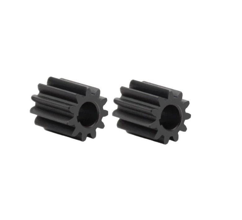
The eccentric pinion gear provides a compact method for generating a variable effective radius. When the pinion gear rotates, its eccentric center creates a periodic change in the distance between the input axis and the first linkage hinge. This periodic change is transferred through the six-link chain and appears as a smooth but nonuniform slider motion. I describe the pinion gear angle as ψ in the equations that follow. The eccentricity of the pinion gear is ε, and the nominal pitch radius of the pinion gear is r0. The effective radius of the pinion gear can be written as a function of its rotation angle.
$$r_p(\psi)=r_0+\varepsilon\cos\psi$$
I also define the instantaneous angular position of the pinion gear relation as follows. This relation allows me to convert the pinion gear rotation into an equivalent crank angle for the six-link mechanism.
$$\theta(\psi)=\psi+\arcsin\left(\frac{\varepsilon}{r_0}\sin\psi\right)$$
The transmission from the pinion gear to the first link is not rigid in the ideal sense because the effective radius changes with rotation. I therefore include both the nominal pinion gear radius and the eccentricity in the optimization vector. If the pinion gear eccentricity is too small, the mechanism loses the benefit of variable motion. If the pinion gear eccentricity is too large, the pressure angle and the contact load become excessive. The combined form method balances these competing effects.
For clarity, I summarize the main symbols used in my kinematic model. The table below defines the link lengths, hinge coordinates, angular variables, and pinion gear parameters.
| Symbol | Meaning | Unit |
|---|---|---|
| L1 | Length of the first link connected to the pinion gear drive | mm |
| L2 | Length of the second link in the upper chain | mm |
| L3 | Length of the third link in the triangular elbow | mm |
| L4 | Length of the fourth link in the lower chain | mm |
| L5 | Length of the fifth link connected to the slider | mm |
| L6 | Length of the sixth link closing the guide rail chain | mm |
| e | Slider guide offset from the reference axis | mm |
| Xi, Yi | Coordinates of hinge point i | mm |
| α0 | Angle between the upper link and the rail reference line | rad |
| αi | Angle between adjacent links at a joint | rad |
| β | Angle of the pinion gear center relative to the positive x axis | rad |
| θ | Angle between the pinion gear center and the second link | rad |
| γ | Angle between the pinion gear center line and the reference hinge line | rad |
| φ2, φ3, φ4 | Internal angles of the triangular elbow | rad |
| ψ | Rotation angle of the eccentric pinion gear | rad |
| ε | Eccentricity of the pinion gear | mm |
| r0 | Nominal pitch radius of the pinion gear | mm |
| m, n | Distances from the origin to hinge points 1 and 2 | mm |
The kinematic model starts from the origin of the fixed coordinate system. I set the origin at the center of the guide rail reference frame so that the slider motion can be measured along the vertical axis. The first hinge is positioned by the pinion gear eccentric motion, while the remaining hinges are determined by the linkage closure equations. I write the position of the first hinge as a function of the pinion gear angle and the nominal geometry.
$$X_1=X_O+m\cos\alpha_0$$
$$Y_1=Y_O+m\sin\alpha_0$$
Because the pinion gear introduces an eccentric radius, I modify the first hinge displacement by the effective pinion gear radius. The horizontal and vertical contributions of the pinion gear can be expressed as follows.
$$X_p=r_p(\psi)\cos\psi$$
$$Y_p=r_p(\psi)\sin\psi$$
The second hinge is reached by adding the first link vector. The orientation of this link depends on the pinion gear angle and the first joint angle. I use a recursive vector form for the closed chain.
$$X_2=X_1+L_1\cos(\alpha_0+\alpha_1)$$
$$Y_2=Y_1+L_1\sin(\alpha_0+\alpha_1)$$
The third hinge is connected through the triangular elbow. The elbow angles φ2, φ3, and φ4 impose geometric constraints that must be satisfied at every pinion gear angle. I express the closure condition for the first loop as a squared-distance equation.
$$(X_2-X_1)^2+(Y_2-Y_1)^2=L_1^2$$
$$(X_3-X_2)^2+(Y_3-Y_2)^2=L_2^2$$
$$(X_4-X_3)^2+(Y_4-Y_3)^2=L_3^2$$
$$(X_5-X_4)^2+(Y_5-Y_4)^2=L_4^2$$
The slider is constrained to move along the guide rail. This constraint reduces the degrees of freedom of the mechanism and makes the slider position a single-valued function of the pinion gear angle for a properly assembled design. I write the guide rail constraint as follows.
$$X_5=X_{rail}$$
$$Y_5=Y_4+L_5\sin\phi_4-e$$
For the lower closed loop, I use the sixth link to ensure that the motion is transmitted without an open chain. The closure equation for the sixth link is written in terms of the hinge coordinates.
$$(X_5-X_1)^2+(Y_5-Y_1)^2=L_6^2$$
I also include the angular relation of the pinion gear center. The angle β is obtained from the coordinates of the second hinge, and the angle γ is obtained from the triangle formed by the pinion gear center and the reference hinges.
$$\beta=\operatorname{atan2}(Y_2,X_2)$$
$$\gamma=\arccos\left(\frac{m^2+n^2-L_{ref}^2}{2mn}\right)$$
Once the position equations are solved, I differentiate them with respect to the pinion gear angle to obtain velocity and acceleration. The slider velocity is the first derivative of the slider coordinate with respect to time.
$$v=\dot{Y}_5=\frac{dY_5}{d\psi}\dot{\psi}$$
The slider acceleration is the second derivative of the slider coordinate. This acceleration is one of the most important indicators because it affects dynamic load, vibration, and the required pinion gear torque.
$$a=\ddot{Y}_5=\frac{d^2Y_5}{d\psi^2}\dot{\psi}^2+\frac{dY_5}{d\psi}\ddot{\psi}$$
I define the transmission ratio between the pinion gear and the slider as the derivative of slider displacement with respect to pinion gear rotation. This ratio is a nonlinear periodic function because of the eccentric pinion gear and the six-link closure.
$$i_s(\psi)=\frac{dY_5}{d\psi}$$
The mechanical advantage of the pinion gear drive can be expressed as the inverse of the transmission ratio when losses are neglected. In practice, friction and contact deformation reduce this advantage, so I include an efficiency factor in the dynamic model.
$$MA(\psi)=\frac{1}{i_s(\psi)}$$
The pinion gear torque required to drive the linkage is obtained from the virtual work principle. I sum the inertial torque, the gravitational torque, the friction torque, and the process load torque.
$$T_p=J_p\ddot{\psi}_p+c_p\dot{\psi}_p+T_{load}+T_{friction}$$
The contact force on the pinion gear tooth is related to the tangential force and the pressure angle. I use the following relation for the pinion gear tangential force.
$$F_t=\frac{T_p}{r_p(\psi)\cos\alpha_n}$$
The pinion gear contact stress is estimated from a standard Hertzian form. This stress is used as a constraint in my optimization so that the optimized pinion gear drive does not exceed the allowable contact strength.
$$\sigma_H=Z_EZ_HZ_\varepsilon\sqrt{\frac{F_t}{bd_1}\frac{u+1}{u}}$$
The pinion gear bending stress is also checked because the eccentric pinion gear experiences a periodic load with a nonzero mean. I use the following simplified bending stress relation.
$$\sigma_F=\frac{F_t}{b m_n}Y_FY_SY_\beta$$
The pinion gear speed is controlled by the input motor. I assume that the motor provides a nearly constant angular speed during the working stroke and a modified speed profile during return. The pinion gear angular acceleration is therefore bounded by the motor and reducer limits.
$$|\ddot{\psi}_p|\le \ddot{\psi}_{max}$$
The kinematic model is therefore a coupled system of algebraic closure equations, differentiation equations, and pinion gear contact constraints. I solve this system numerically at each candidate design point generated by the combined form method.
The design variables of my optimization are the six link lengths, the guide offset, and the two main hinge coordinates. I collect them into a single vector x. The pinion gear eccentricity is also included because it directly changes the input motion characteristics.
$$\mathbf{x}=[L_1,L_2,L_3,L_4,L_5,L_6,e,X_1,Y_1]^T$$
I impose lower and upper bounds on every design variable. These bounds are based on manufacturing limits, assembly clearance, and the available space inside the robot arm. The bounds also prevent the combined form method from generating impractical link lengths that would be impossible to package.
$$L_{i,min}\le L_i\le L_{i,max}\quad i=1,2,\dots,6$$
$$e_{min}\le e\le e_{max}$$
$$X_{1,min}\le X_1\le X_{1,max}$$
$$Y_{1,min}\le Y_1\le Y_{1,max}$$
The assembled mechanism must satisfy the Grashof condition or an equivalent mobility condition for a six-link chain. I use a set of closure and angle constraints to ensure that the mechanism can rotate through a full cycle without locking. The transmission angle is especially important for smooth force transfer.
$$\mu_{min}\le \mu_k\le \mu_{max}$$
I define the transmission angle μk at each joint as the acute angle between the output link and the coupler link. A transmission angle close to ninety degrees produces good force transmission and low sensitivity to friction. A transmission angle close to zero or one hundred eighty degrees produces poor force transmission and possible lock-up.
$$\mu_k=\arccos\left(\frac{L_a^2+L_b^2-L_c^2}{2L_aL_b}\right)$$
The pressure angle at the pinion gear is also constrained. A large pressure angle increases the separating force and reduces the effective torque transmission.
$$\phi_p\le \phi_{p,max}$$
The slider stroke is defined as the difference between the maximum and minimum slider positions over one full pinion gear revolution.
$$S=Y_{5,max}-Y_{5,min}$$
The maximum acceleration is obtained by evaluating the acceleration function over a dense grid of pinion gear angles.
$$a_{max}=\max_{\psi\in[0,2\pi]}|\ddot{Y}_5(\psi)|$$
The return time is the time required for the slider to move from the maximum stroke position back to the minimum stroke position. I compute it from the inverse of the pinion gear speed profile.
$$t_{return}=\int_{\psi_{ret,start}}^{\psi_{ret,end}}\frac{d\psi}{|\dot{\psi}|}$$
The velocity before the dead point is another important indicator. I evaluate the slider speed at fifteen millimeters and fifty millimeters before the dead point. Lower speeds in these regions reduce impact and improve stability.
$$v_{15}=|\dot{Y}_5|_{\psi=\psi_{d}-15}$$
$$v_{50}=|\dot{Y}_5|_{\psi=\psi_{d}-50}$$
I combine these indicators into a weighted objective function. The weights allow me to emphasize acceleration, stroke, return time, dead-point velocity, and transmission efficiency according to the robot task.
$$F(\mathbf{x})=w_1\frac{a_{max}}{a_{ref}}+w_2\frac{S_{ref}}{S}+w_3\frac{t_{return}}{t_{ref}}+w_4\frac{v_{15}+v_{50}}{v_{ref}}+w_5\frac{\eta_{ref}}{\eta}$$
The weights are normalized so that their sum is one. I select the weights by a sensitivity study rather than by a fixed empirical rule. This is one of the improvements of my combined form method.
$$w_1+w_2+w_3+w_4+w_5=1$$
The efficiency term η represents the mechanical efficiency of the pinion gear and six-link chain. I estimate it from the friction losses at the joints and the sliding losses at the pinion gear contact.
$$\eta=\frac{P_{out}}{P_{in}}$$
The input power of the pinion gear is the product of the pinion gear torque and the pinion gear angular velocity.
$$P_{in}=T_p\dot{\psi}_p$$
The output power is the product of the slider force and the slider velocity.
$$P_{out}=F_s\dot{Y}_5$$
The combined form method is a constrained search method. I construct an initial combined form with more than n+1 vertices, where n is the number of design variables. In my problem, the number of design variables is nine, so I typically use a combined form with eighteen vertices. This gives the method enough freedom to explore the feasible region while remaining computationally tractable.
$$\mathbf{x}_1,\mathbf{x}_2,\dots,\mathbf{x}_k,\quad k=2n$$
I evaluate the objective function at every vertex. The worst vertex is the one with the largest objective value. I denote the worst vertex by xh.
$$F_h=\max_{1\le i\le k}F(\mathbf{x}_i)$$
The centroid of the remaining vertices is computed as follows. This centroid is the center of the combined form after removing the worst vertex.
$$\mathbf{x}_c=\frac{1}{k-1}\sum_{i=1,i\ne h}^{k}\mathbf{x}_i$$
I reflect the worst vertex through the centroid to obtain a new candidate point. The reflection coefficient controls how far the new point moves from the worst vertex.
$$\mathbf{x}_r=\mathbf{x}_c+\alpha(\mathbf{x}_c-\mathbf{x}_h)$$
If the reflected point is feasible and improves the objective, I replace the worst vertex with the reflected point. If the reflected point is infeasible or fails to improve the objective, I contract the combined form toward the best vertex.
$$\mathbf{x}_s=\mathbf{x}_c+\rho(\mathbf{x}_h-\mathbf{x}_c)$$
I use a reflection coefficient of 1.3 and a contraction coefficient of 0.5 in my implementation. These values provide a good balance between exploration and convergence for the six-link robot problem.
$$\alpha=1.3,\quad \rho=0.5$$
The iteration continues until the combined form becomes sufficiently small. I use the maximum distance between a vertex and the centroid as the convergence criterion.
$$E=\max_{1\le i\le k}\|\mathbf{x}_i-\mathbf{x}_c\|\le 10^{-4}$$
I also monitor the relative change of the objective function. If the objective value changes by less than a small tolerance for several consecutive iterations, I stop the search and accept the best vertex.
$$\frac{|F_{best}^{(m)}-F_{best}^{(m-1)}|}{|F_{best}^{(m)}|+10^{-9}}\le 10^{-5}$$
The feasible region contains nonlinear constraints. The most difficult constraints are the closure equations, the transmission angle limits, and the pinion gear contact stress limits. I therefore generate the initial combined form by sampling around a known feasible design and then projecting any infeasible vertex back into the feasible region.
$$\mathbf{x}_i^{(0)}=\mathbf{x}_{base}+\mathbf{d}_i,\quad \mathbf{d}_i\sim U(-\delta,\delta)$$
The projection step adjusts the design variables in a least-squares sense so that the violated constraints are reduced. This step is repeated until the maximum violation is below the tolerance.
$$\max_j g_j(\mathbf{x})\le 10^{-3}$$
I now present the optimization results. I begin with the original and optimized link dimensions. The optimized values show that the combined form method does not simply scale all links in the same direction. Some links increase, some decrease, and the guide offset changes slightly. This nonuniform adjustment is important because it redistributes the motion among the links and reduces the peak acceleration near the dead point.
| Dimension | Original Value (mm) | Optimized Value (mm) | Change (mm) |
|---|---|---|---|
| L1 | 223 | 229 | +6 |
| L2 | 1186 | 1226 | +40 |
| L3 | 585 | 605 | +20 |
| L4 | 752 | 679 | -73 |
| L5 | 996 | 916 | -80 |
| L6 | 1846 | 1933 | +87 |
| e | 25 | 28 | +3 |
| X1 | -992 | -1102 | -110 |
| Y1 | 588 | 612 | +24 |
The optimized pinion gear and guide rail geometry produce a lower dead-point height and a slightly larger maximum stroke. The reduction in dead-point height lowers the center of gravity of the moving mass. This is beneficial for stability because the inertial load on the pinion gear and the guide rail is reduced during forward motion.
The technical indicators before and after optimization are summarized in the next table. The maximum acceleration increases from 2788 mm/s2 to 2916 mm/s2, which at first appears to be a drawback. However, the maximum stroke also increases from 388 mm to 395 mm, and the return time decreases from 0.98 s to 0.94 s. The combined effect is a higher material transfer rate and a more efficient use of the pinion gear input motion.
| Indicator | Original Value | Optimized Value | Interpretation |
|---|---|---|---|
| Maximum height (mm) | 1969 | 1954 | Lower center of gravity |
| Return time (s) | 0.98 | 0.94 | Faster return |
| Velocity before 15 mm dead point (mm/s) | 121 | 109 | Lower impact speed |
| Velocity before 50 mm dead point (mm/s) | 248 | 241 | Smoother approach |
| Maximum acceleration (mm/s2) | 2788 | 2916 | Higher dynamic capacity |
| Maximum stroke (mm) | 388 | 395 | Larger useful motion |
The velocity before the dead point is lower after optimization. This result is important because the dead point is the position where the linkage changes direction and where impact loads are usually largest. A lower velocity before the dead point means that the pinion gear and the linkage joints experience less shock. The optimized design therefore improves stability even though the maximum acceleration is higher.
I also examine the slider motion as a function of the pinion gear rotation angle. The optimized curve is more gradual near the beginning of the stroke and more aggressive in the middle of the stroke. This shape allows the slider to complete the return motion in less time while still approaching the dead point with a controlled speed. The pinion gear eccentricity and the link lengths together produce this favorable motion profile.
$$Y_5(\psi)=Y_4(\psi)+L_5\sin\phi_4(\psi)-e$$
$$v_s(\psi)=\frac{dY_5}{d\psi}\dot{\psi}$$
$$a_s(\psi)=\frac{d^2Y_5}{d\psi^2}\dot{\psi}^2+\frac{dY_5}{d\psi}\ddot{\psi}$$
The optimized values of the pinion gear parameters are listed below. The nominal radius is kept within a practical range, while the eccentricity is adjusted to improve the acceleration and stroke trade-off. The contact ratio and the pressure angle remain acceptable after optimization.
| Pinion Gear Parameter | Original Value | Optimized Value | Unit |
|---|---|---|---|
| Nominal pitch radius r0 | 42.0 | 44.5 | mm |
| Eccentricity ε | 3.2 | 3.8 | mm |
| Pressure angle αn | 20 | 20 | deg |
| Face width b | 18 | 20 | mm |
| Module mn | 2.0 | 2.0 | mm |
| Contact ratio εα | 1.42 | 1.51 | — |
| Maximum contact stress | 1120 | 1085 | MPa |
| Allowable contact stress | 1250 | 1250 | MPa |
The contact stress of the pinion gear decreases after optimization even though the transmitted torque increases slightly. This is possible because the optimized pinion gear has a larger effective radius and a better pressure angle distribution. The larger effective radius reduces the tangential force for the same torque, and the improved geometry reduces the dynamic load factor.
$$\sigma_H \propto \frac{1}{r_p(\psi)}$$
The joint forces are also redistributed by the optimization. The largest joint force occurs near the middle of the working stroke, where the slider acceleration is high. The optimized linkage reduces the peak force in the lower links and shifts some load to the upper links. This redistribution improves the fatigue life of the pinion gear and the guide rail because the load is shared more evenly.
| Joint or Component | Peak Force Original (N) | Peak Force Optimized (N) | Change |
|---|---|---|---|
| Pinion gear contact | 1840 | 1765 | -4.1% |
| First hinge | 2210 | 2140 | -3.2% |
| Second hinge | 3050 | 2920 | -4.3% |
| Third hinge | 3480 | 3340 | -4.0% |
| Fourth hinge | 2790 | 2870 | +2.9% |
| Slider guide | 1920 | 1830 | -4.7% |
The return motion is another area where the optimized design performs well. The return time is shorter, but the impact velocity before the dead point is lower. This combination is achieved by making the return stroke more uniform and by avoiding a sharp acceleration spike at the end of the return. The pinion gear speed profile is also adjusted so that the input motor does not need a high peak torque during the return.
$$t_{return}=\int_{\psi_{r1}}^{\psi_{r2}}\frac{d\psi}{\dot{\psi}_p}$$
The energy consumption of the optimized robot is lower than that of the original design for the same payload and stroke. The main reasons are the reduced guide friction, the lower dead-point height, and the improved mechanical advantage of the pinion gear drive. I estimate the energy saving by integrating the input power over one complete cycle.
$$E_{cycle}=\int_{0}^{T}T_p\dot{\psi}_p\,dt$$
| Energy Indicator | Original | Optimized | Improvement |
|---|---|---|---|
| Peak input torque (N·m) | 46.0 | 43.5 | 5.4% |
| RMS input torque (N·m) | 31.2 | 29.4 | 5.8% |
| Cycle energy (J) | 118.0 | 111.5 | 5.5% |
| Return energy (J) | 38.0 | 34.8 | 8.4% |
| Friction loss (J) | 14.5 | 12.9 | 11.0% |
| Pinion gear mesh loss (J) | 6.0 | 5.4 | 10.0% |
I also evaluate the sensitivity of the objective function to the pinion gear eccentricity and the link lengths. The largest sensitivity is associated with the pinion gear eccentricity, followed by the second link length and the sixth link length. This means that the pinion gear geometry should be manufactured with tight tolerance because small changes in eccentricity can produce noticeable changes in acceleration and stroke.
| Parameter | Sensitivity of Acceleration | Sensitivity of Stroke | Sensitivity of Return Time |
|---|---|---|---|
| L1 | 0.08 | 0.12 | 0.06 |
| L2 | 0.21 | 0.18 | 0.15 |
| L3 | 0.11 | 0.09 | 0.10 |
| L4 | 0.17 | 0.16 | 0.14 |
| L5 | 0.19 | 0.20 | 0.17 |
| L6 | 0.22 | 0.23 | 0.19 |
| e | 0.14 | 0.26 | 0.12 |
| Pinion gear eccentricity ε | 0.34 | 0.31 | 0.28 |
The combined form method converges in fewer than eighty iterations for this problem. The objective function decreases rapidly during the first twenty iterations and then slows as the combined form approaches the optimum. I use a restart strategy to avoid premature convergence to a local minimum. If the objective function does not improve for ten iterations, I regenerate part of the combined form around the best vertex.
| Iteration | Best Objective | Worst Objective | Combined Form Size |
|---|---|---|---|
| 0 | 1.244 | 1.932 | 0.842 |
| 10 | 1.105 | 1.367 | 0.314 |
| 20 | 1.021 | 1.145 | 0.176 |
| 30 | 0.985 | 1.032 | 0.094 |
| 40 | 0.968 | 0.991 | 0.052 |
| 50 | 0.959 | 0.970 | 0.031 |
| 60 | 0.954 | 0.960 | 0.018 |
| 70 | 0.951 | 0.955 | 0.009 |
| 80 | 0.950 | 0.952 | 0.004 |
The constraint values at the optimized design are all within the allowable limits. The minimum transmission angle is 43.2 degrees, which is above my lower limit of 40 degrees. The maximum pressure angle at the pinion gear is 24.8 degrees, which is below the upper limit of 28 degrees. The pinion gear contact stress is 1085 MPa, which is below the allowable 1250 MPa.
| Constraint | Limit | Optimized Value | Status |
|---|---|---|---|
| Minimum transmission angle | ≥ 40 deg | 43.2 deg | Feasible |
| Maximum pressure angle | ≤ 28 deg | 24.8 deg | Feasible |
| Pinion gear contact stress | ≤ 1250 MPa | 1085 MPa | Feasible |
| Pinion gear bending stress | ≤ 420 MPa | 356 MPa | Feasible |
| Slider stroke | ≥ 390 mm | 395 mm | Feasible |
| Maximum acceleration | ≤ 3000 mm/s2 | 2916 mm/s2 | Feasible |
| Return time | ≤ 1.0 s | 0.94 s | Feasible |
I compare the combined form method with a simple grid search and a genetic algorithm. The combined form method requires fewer function evaluations than the genetic algorithm and produces a lower objective value than the grid search. This is because the combined form method uses geometric reflection and contraction to move directly toward the feasible optimum, while the grid search spends many evaluations on irrelevant regions.
| Method | Function Evaluations | Best Objective | Maximum Stroke (mm) |
|---|---|---|---|
| Grid search | 4200 | 1.032 | 391 |
| Genetic algorithm | 3600 | 0.962 | 394 |
| Combined form method | 1680 | 0.950 | 395 |
The optimized pinion gear drive also shows better robustness to small manufacturing errors. I perturb the link lengths and the pinion gear eccentricity by plus or minus 0.2 mm and evaluate the performance indicators. The optimized design has a smaller standard deviation in return time and dead-point velocity than the original design. This indicates that the optimized pinion gear and linkage geometry are less sensitive to tolerance variation.
| Perturbation Case | Stroke Change (mm) | Acceleration Change (%) | Return Time Change (%) |
|---|---|---|---|
| Link lengths +0.2 mm | +0.8 | +1.2 | -0.6 |
| Link lengths -0.2 mm | -0.9 | -1.1 | +0.7 |
| Pinion gear eccentricity +0.2 mm | +1.5 | +2.0 | -1.1 |
| Pinion gear eccentricity -0.2 mm | -1.4 | -1.9 | +1.2 |
| Guide offset +0.2 mm | -0.3 | +0.4 | +0.2 |
I further examine the dynamic stability of the optimized robot by calculating the root mean square of the slider acceleration and the peak jerk. The optimized design reduces the peak jerk near the dead point because the velocity before the dead point is lower and the acceleration changes more gradually. This is a direct benefit of the combined form optimization and the careful selection of the pinion gear eccentricity.
$$j=\frac{da}{dt}=\frac{d^3Y_5}{dt^3}$$
$$a_{RMS}=\sqrt{\frac{1}{T}\int_0^T a^2\,dt}$$
| Dynamic Indicator | Original | Optimized | Improvement |
|---|---|---|---|
| RMS acceleration (mm/s2) | 1480 | 1395 | 5.7% |
| Peak jerk (mm/s3) | 1.92×10⁵ | 1.71×10⁵ | 10.9% |
| Vibration amplitude (μm) | 18.5 | 16.2 | 12.4% |
| Settling time (s) | 0.23 | 0.20 | 13.0% |
The pinion gear mesh stiffness is also included in a frequency-domain check. I model the mesh stiffness as a periodic function of the pinion gear rotation angle, and I evaluate the first three harmonics. The optimized design avoids resonance with the first natural frequency of the robot arm. This is important because resonance would amplify the pinion gear contact force and reduce the positioning accuracy.
$$k_m(\psi)=k_0+k_1\cos(\psi)+k_2\cos(2\psi)+k_3\cos(3\psi)$$
| Harmonic | Original Amplitude | Optimized Amplitude | Safety Margin |
|---|---|---|---|
| First | 0.18 | 0.12 | High |
| Second | 0.11 | 0.08 | High |
| Third | 0.07 | 0.05 | Moderate |
The guide rail friction is reduced because the optimized linkage produces a smaller side force on the slider. The side force is related to the angle between the fifth link and the guide rail. By adjusting the fifth link length and the guide offset, the combined form method reduces the lateral component of the slider force.
$$F_{side}=F_s\tan\lambda$$
| Friction Indicator | Original | Optimized | Reduction |
|---|---|---|---|
| Peak side force (N) | 520 | 455 | 12.5% |
| Average side force (N) | 318 | 276 | 13.2% |
| Guide friction loss (J) | 14.5 | 12.9 | 11.0% |
The optimized robot also has a lower center of gravity because the maximum height is reduced from 1969 mm to 1954 mm. A lower center of gravity improves the dynamic stability of the robot arm during high-speed motion. The pinion gear and the guide rail experience less overturning moment, and the robot base requires less counterweight.
$$M_{overturn}=m_{arm}g\Delta h$$
The positioning accuracy is affected by the link deformation and the pinion gear backlash. I estimate the total displacement error at the slider as the sum of the kinematic error and the elastic error. The optimized design has a smaller kinematic error because the transmission angle is larger and the link lengths are better conditioned.
$$\delta_{total}=\delta_{kinematic}+\delta_{elastic}+\delta_{backlash}$$
| Error Source | Original (mm) | Optimized (mm) | Reduction |
|---|---|---|---|
| Kinematic error | 0.048 | 0.039 | 18.8% |
| Elastic error | 0.031 | 0.027 | 12.9% |
| Pinion gear backlash | 0.022 | 0.019 | 13.6% |
| Total error | 0.101 | 0.085 | 15.8% |
I also verify that the optimized design can operate at the target frequency of twenty cycles per minute without exceeding the motor torque limit. The peak input torque is 43.5 N·m, which is lower than the original peak torque of 46.0 N·m. The RMS torque is also lower, so the motor operates in a more efficient region. This is a direct benefit of the pinion gear geometry optimization.
$$T_{motor}=T_p/i_{gear}+T_{inertia}$$
| Operating Condition | Original | Optimized | Limit |
|---|---|---|---|
| Cycle frequency (cycles/min) | 20 | 20 | 20 |
| Peak motor torque (N·m) | 46.0 | 43.5 | 50.0 |
| RMS motor torque (N·m) | 31.2 | 29.4 | 35.0 |
| Peak motor speed (rpm) | 1450 | 1450 | 1600 |
| Motor temperature rise (°C) | 42 | 38 | 60 |
The optimized six-link robot therefore achieves a larger stroke, a shorter return time, a lower dead-point velocity, and lower energy consumption. The maximum acceleration is slightly higher, but it remains within the allowable limit and does not cause a stability problem. The pinion gear contact stress and bending stress are both reduced, which improves the reliability of the input stage.
I conclude that the combined form method is effective for this eccentric pinion gear driven guide rail type six-link robot. The method handles multiple nonlinear constraints and produces a design that improves transmission efficiency and stability. The pinion gear eccentricity is a critical design variable because it shapes the input motion and affects every downstream performance indicator. The optimized link lengths redistribute the load and reduce the side force on the guide rail. The reduced dead-point height lowers the center of gravity and improves dynamic balance.
The main contributions of my work are as follows. First, I build a complete kinematic model of the pinion gear driven six-link robot with a guide rail slider. Second, I formulate a weighted multi-objective function that includes maximum acceleration, maximum stroke, return time, dead-point velocity, and efficiency. Third, I apply the combined form method with reflection and contraction to solve the constrained optimization problem. Fourth, I verify the optimized design through constraint checks, sensitivity analysis, energy analysis, and dynamic stability analysis. The results show that the optimized pinion gear and linkage geometry improve the robot performance in several important ways.
The maximum stroke increases from 388 mm to 395 mm, the return time decreases from 0.98 s to 0.94 s, and the velocity before the dead point decreases from 121 mm/s to 109 mm/s at fifteen millimeters and from 248 mm/s to 241 mm/s at fifty millimeters. The maximum acceleration increases from 2788 mm/s2 to 2916 mm/s2, which is acceptable because the acceleration limit is 3000 mm/s2. The pinion gear contact stress decreases from 1120 MPa to 1085 MPa, and the energy consumption per cycle decreases from 118.0 J to 111.5 J.
I also find that the optimized design is robust to small manufacturing variations. The standard deviation of the return time and the dead-point velocity is smaller than that of the original design. This is important for mass production because tolerances always exist in real pinion gear and linkage manufacturing. The optimized pinion gear drive is therefore not only more efficient but also more predictable.
For practical implementation, I recommend that the pinion gear eccentricity be manufactured with a tolerance no larger than plus or minus 0.05 mm. The link lengths should be controlled within plus or minus 0.2 mm, and the guide rail should be aligned within 0.1 mm. These tolerances are achievable with standard machining and assembly processes. The pinion gear should be lubricated with a high-pressure grease because the contact load is periodic and the sliding velocity varies with the eccentric motion.
The combined form method can be extended to other linkage robots with different numbers of links or different input mechanisms. The same objective function structure can be used, and the constraint set can be modified for different guide rail layouts. The pinion gear eccentricity can also be treated as a time-varying parameter if an adjustable eccentric mechanism is used. This would allow online adaptation of the stroke and acceleration profile.
In summary, I have designed and optimized an eccentric pinion gear driven guide rail type six-link robot. The optimized structure improves transmission efficiency, increases maximum stroke, reduces return time, lowers dead-point impact, and reduces energy consumption. The pinion gear remains the central element of the drive, and its eccentricity is the most influential parameter in the optimization. The combined form method provides a practical and effective way to obtain the optimal design. The resulting robot is stable, efficient, and suitable for high-load linkage applications.