
I propose a hybrid digital-model-driven fault diagnosis framework for wind turbine planetary gearboxes, with particular attention to the pinion gears that operate between the sun gear and the ring gear. In my view, the central difficulty in real wind turbine condition monitoring is not the lack of sensing data in general, but the extreme scarcity of high-quality labeled fault data for pinion gears and other critical rotating components. A wind turbine planetary gearbox usually runs in a healthy state for long periods, and when a fault develops, the control system may shut the machine down before a rich, well-labeled fault record can be collected. As a result, healthy data are abundant while fault data for pinion gears, sun gears, ring gears, and bearings are limited. Deep diagnosis models trained only on such imbalanced records tend to overfit the healthy class and produce unreliable decisions for rare but dangerous faults.
To address this problem, I combine a high-fidelity dynamic model of a wind turbine planetary gearbox with a domain-shared residual network, a local distribution alignment module, and a Kolmogorov-Arnold network classifier. The dynamic model generates pseudo-fault data for pinion gears and other geared components, while the network learns transferable physical features from both pseudo-fault data and measured data. I use a convolutional block attention mechanism to strengthen feature extraction, a local maximum mean discrepancy to align fault-category-level distributions, and a Kolmogorov-Arnold network to improve classification of complex nonlinear relationships. The framework is validated on two experimental planetary gearbox systems under multiple speed conditions. The results show that my method maintains high diagnostic accuracy when real fault samples are scarce, and it outperforms several classical data-level and algorithm-level approaches.
1. Motivation and Problem Statement
Wind power has become a major pillar of low-carbon electricity generation. Doubly fed wind turbines and other mainstream configurations must operate in harsh, variable, and often remote environments. The planetary gearbox is one of the most important and most vulnerable subsystems in the drivetrain. It transfers torque from the low-speed rotor to the high-speed generator stage, and it contains multiple pinion gears that mesh simultaneously with the sun gear and the ring gear. Because of this multi-mesh configuration, the vibration response of the planetary gearbox is complex, modulated, and strongly influenced by time-varying mesh stiffness, load sharing among pinion gears, carrier motion, and manufacturing or assembly errors.
Faults in pinion gears, sun gears, ring gears, and bearings can reduce power production, increase maintenance cost, and even cause catastrophic downtime. Therefore, accurate fault diagnosis of the wind turbine planetary gearbox is essential. Deep learning has shown strong potential in this field because it can automatically extract fault-sensitive features from raw vibration signals. However, most successful deep diagnosis models assume that a large number of labeled fault samples are available. In real wind turbine operation, this assumption is rarely satisfied. The gearbox remains healthy for most of its service life, and fault records are few, unbalanced, and sometimes unlabeled. The scarcity of fault data is especially severe for pinion gears because a single damaged pinion gear may trigger an immediate shutdown, leaving only a short and noisy record.
Existing solutions can be broadly divided into data-level methods and algorithm-level methods. Data-level methods include oversampling, undersampling, and generative data augmentation. Oversampling can cause overfitting to minority fault samples, while undersampling can discard useful information from the majority healthy class. Generative adversarial networks can synthesize fault samples, but they often suffer from unstable training and mode collapse, and the generated data may not contain complete physical fault characteristics. Algorithm-level methods adjust the loss function or class weights to reduce the bias toward the majority class. These methods can be effective when some fault samples exist, but when fault data are extremely scarce, the decision boundary remains unreliable and generalization is limited.
My motivation is to use physical knowledge from a dynamic model to supplement the scarce measured fault data. Instead of relying only on measured records, I build a high-fidelity model of the wind turbine planetary gearbox and generate pseudo-fault data for pinion gears and other components. Then I align the pseudo-fault distribution with the real fault distribution at the fault-category level. This hybrid strategy uses both physical simulation and data-driven learning, and it reduces the dependence on large real fault datasets. The main contributions of my work are as follows.
| Contribution | Description |
|---|---|
| High-fidelity dynamic model | I use a lumped-parameter model with time-varying mesh stiffness to simulate healthy and faulty states of the planetary gearbox, including pinion gears, sun gear, ring gear, and carrier. |
| Pseudo-fault data generation | I generate pseudo-fault samples for missing tooth, broken tooth, and crack conditions to supplement scarce real fault samples. |
| Domain-shared residual feature extractor | I design a residual network with convolutional block attention to extract shared physical features from pseudo and measured data. |
| Local distribution alignment | I introduce local maximum mean discrepancy to align pseudo-fault and real-fault features at the fault-category level. |
| Kolmogorov-Arnold classifier | I use a Kolmogorov-Arnold network to improve nonlinear classification and noise suppression. |
| Experimental validation | I validate the method on two planetary gearbox test systems under multiple speed conditions and compare it with classical methods. |
2. High-Fidelity Dynamic Modeling of the Planetary Gearbox with Pinion Gears
I adopt the lumped-parameter method to model the wind turbine planetary gearbox because it is computationally efficient and can be combined with data-driven diagnosis. The model includes one sun gear, one carrier, one ring gear, and several equally spaced pinion gears. Each component has two translational degrees of freedom and one rotational degree of freedom. The pinion gears mesh with the sun gear and the ring gear, and their dynamic interactions are represented by spring-damper elements. The time-varying mesh stiffness is calculated by the potential energy method, which allows me to introduce different fault forms into the model.
The dynamic equations of the sun gear can be written as:
$$
\begin{aligned}
m_s\left(\ddot{x}_s – x_s\omega_c^2 – 2\dot{y}_s\omega_c – y_s\dot{\omega}_c\right) + k_s x_s + c_s\dot{x}_s + \sum_{n=1}^{N} F_{spn}\cos\psi_{sn} &= 0, \\
m_s\left(\ddot{y}_s – y_s\omega_c^2 + 2\dot{x}_s\omega_c + x_s\dot{\omega}_c\right) + k_s y_s + c_s\dot{y}_s + \sum_{n=1}^{N} F_{spn}\sin\psi_{sn} &= 0, \\
\frac{J_s}{r_s}\ddot{\theta}_s + \sum_{n=1}^{N} F_{spn} &= \frac{T_i}{r_s}.
\end{aligned}
$$
The carrier equations are:
$$
\begin{aligned}
m_c\left(\ddot{x}_c – x_c\omega_c^2 – 2\dot{y}_c\omega_c – y_c\dot{\omega}_c\right) + k_{cx}x_c + c_c\dot{x}_c – \sum_{n=1}^{N} F_{cpnx} &= 0, \\
m_c\left(\ddot{y}_c – y_c\omega_c^2 + 2\dot{x}_c\omega_c + x_c\dot{\omega}_c\right) + k_{cy}y_c + c_c\dot{y}_c – \sum_{n=1}^{N} F_{cpny} &= 0, \\
\frac{J_c}{r_c}\ddot{\theta}_c + \sum_{n=1}^{N} F_{cpnx}\sin\psi_n – \sum_{n=1}^{N} F_{cpny}\cos\psi_n &= \frac{T_o}{r_c}.
\end{aligned}
$$
The ring gear equations are:
$$
\begin{aligned}
m_r\left(\ddot{x}_r – x_r\omega_c^2 – 2\dot{y}_r\omega_c – y_r\dot{\omega}_c\right) + c_r\dot{x}_r + k_r x_r + \sum_{n=1}^{N} F_{rpn}\cos\psi_{rpn} &= 0, \\
m_r\left(\ddot{y}_r – y_r\omega_c^2 + 2\dot{x}_r\omega_c + x_r\dot{\omega}_c\right) + c_r\dot{y}_r + k_r y_r + \sum_{n=1}^{N} F_{rpn}\sin\psi_{rpn} &= 0, \\
J_r\ddot{\theta}_r + c_{rt}\dot{\theta}_r + k_{rt}\theta_r + r_r\sum_{n=1}^{N} F_{rpn} &= 0.
\end{aligned}
$$
The pinion gear equations are:
$$
\begin{aligned}
m_{pn}\left(\ddot{x}_{pn} – x_{pn}\omega_c^2 – 2\dot{y}_{pn}\omega_c – y_{pn}\dot{\omega}_c\right) + F_{cpnx} – \left(F_{spn} – F_{rpn}\right)\cos\alpha &= 0, \\
m_{pn}\left(\ddot{y}_{pn} – y_{pn}\omega_c^2 + 2\dot{x}_{pn}\omega_c + x_{pn}\dot{\omega}_c\right) + F_{cpny} – \left(F_{spn} + F_{rpn}\right)\sin\alpha &= 0, \\
\frac{J_{pn}}{r_p}\ddot{\theta}_{pn} + F_{spn} – F_{rpn} &= 0.
\end{aligned}
$$
In these equations, \(m_l\) is the mass of a component, \(k_l\) is a support stiffness, \(c_l\) is a support damping, \(J_l\) is a rotary inertia, \(r_l\) is a base circle radius, \(\omega_c\) is the carrier angular speed, \(T_i\) is the input torque, \(T_o\) is the load torque, and \(\alpha\) is the pressure angle. The index \(n\) denotes a pinion gear, and \(N\) is the number of pinion gears. The angular position of each pinion gear is \(\psi_n = 2(n-1)\pi/N\). These equations allow me to simulate the dynamic response of the planetary gearbox with multiple pinion gears under healthy and faulty conditions.
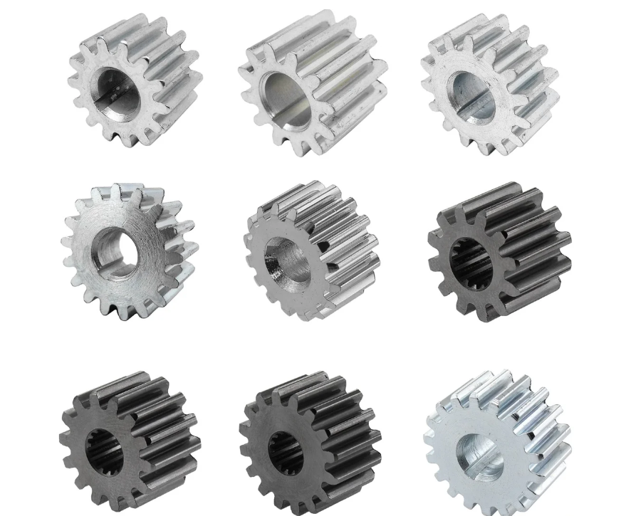
The time-varying mesh stiffness is a key internal excitation. I calculate it using the potential energy method, which decomposes the total mesh stiffness into Hertzian contact stiffness, bending stiffness, axial compression stiffness, shear stiffness, and fillet-foundation stiffness. The combined mesh stiffness for a gear pair is:
$$
k = \sum_{i=1}^{2}\left(
\frac{1}{k_h} +
\frac{1}{k_{b1,i}} +
\frac{1}{k_{s1,i}} +
\frac{1}{k_{a1,i}} +
\frac{1}{k_{f1,i}} +
\frac{1}{k_{b2,i}} +
\frac{1}{k_{s2,i}} +
\frac{1}{k_{a2,i}} +
\frac{1}{k_{f2,i}}
\right)^{-1}.
$$
For external meshing, the two bodies are the sun gear and a pinion gear. For internal meshing, the two bodies are a pinion gear and the ring gear. When the sun gear has a missing tooth, only one tooth pair may carry the load during part of the mesh cycle, so the stiffness calculation must consider single-pair contact. When the sun gear has a broken tooth, the contact area and the effective tooth profile change, which alters the mesh stiffness. When the sun gear has a crack, the crack depth and angle affect the bending and shear stiffness, and therefore the time-varying mesh stiffness. By inserting these fault-dependent stiffness values into the dynamic equations, I obtain simulated vibration responses for different fault types of pinion gears and sun gears.
The main parameters used in my dynamic model are listed in Table 1. These parameters are selected to represent a typical small-scale planetary gearbox used in wind turbine drivetrain experiments. The pinion gears have 36 teeth, the sun gear has 28 teeth, and the ring gear has 100 teeth. The module and pressure angle are kept consistent across the gear pairs.
| Parameter | Sun gear | Pinion gears | Ring gear | Carrier |
|---|---|---|---|---|
| Number of teeth | 28 | 36 | 100 | — |
| Module (mm) | 1.1 | 1.1 | 1.1 | — |
| Pressure angle (deg) | 20 | 20 | 20 | — |
| Face width (mm) | 10 | 10 | 10 | — |
| Mass (kg) | 0.700 | 1.822 | 5.982 | 10.000 |
The sun gear rotation frequency is:
$$
f_s = \frac{n}{60},
$$
where \(n\) is the input speed in revolutions per minute. The gear mesh frequency is:
$$
f_m = \frac{z_s z_r}{60(z_s + z_r)}n,
$$
where \(z_s\) is the number of sun gear teeth and \(z_r\) is the number of ring gear teeth. The local fault characteristic frequency is:
$$
f_{st} = \frac{f_m}{z_s}.
$$
For a missing-tooth fault, the simulated time-domain signal shows periodic impulses, and the frequency spectrum is dominated by the mesh frequency \(f_m\) and its harmonics \(n f_m\). The sidebands around these harmonics reflect the modulation caused by the faulty pinion gears and the sun gear. In my validation, the theoretical mesh frequency for a representative speed is approximately 106.3 Hz. The simulated response has a peak near 106 Hz, and the measured response has a peak near 107.99 Hz. These values are close, which confirms that my dynamic model captures the main frequency characteristics of the real planetary gearbox. The peak amplitudes of the simulated and measured signals are also in the same order of magnitude, and both show impulsive behavior for missing-tooth and broken-tooth conditions. This agreement supports the use of the model as a source of pseudo-fault data for pinion gears and other components.
3. Domain-Shared Residual KAN Network
After generating pseudo-fault data, I need a diagnosis network that can transfer knowledge from the simulated domain to the real domain. I design a domain-shared residual KAN network composed of a feature extractor and a classifier. The feature extractor is shared between the source domain, which contains pseudo-fault data, and the target domain, which contains real measured fault data. This weight sharing encourages the network to learn features that are physically meaningful for both domains. The classifier uses a Kolmogorov-Arnold network to model complex nonlinear relationships and to improve noise robustness.
3.1 Domain-Shared Residual Feature Extractor with Attention
I use a residual network as the backbone because residual connections alleviate gradient degradation in deep networks. Each residual block contains convolutional layers, batch normalization, a nonlinear activation function, and a shortcut connection. I insert a convolutional block attention module into the residual blocks to enhance fault-sensitive feature extraction. The attention module has two parts: channel attention and spatial attention. Channel attention adaptively reweights feature channels, and spatial attention highlights informative spatial regions. This is important for planetary gearbox signals because the vibration response contains contributions from multiple pinion gears, and the fault-related impulses may be weak and localized in time.
The channel attention can be written as:
$$
M_c(F) = \sigma\left(MLP(AvgPool(F)) + MLP(MaxPool(F))\right),
$$
where \(F\) is the input feature map, \(AvgPool\) and \(MaxPool\) denote average pooling and maximum pooling, \(MLP\) is a shared multilayer perceptron, and \(\sigma\) is the sigmoid function. The spatial attention is:
$$
M_s(F) = \sigma\left(f^{7\times 7}\left([AvgPool(F); MaxPool(F)]\right)\right),
$$
where \(f^{7\times 7}\) is a convolution with a \(7\times 7\) kernel, and \([\cdot;\cdot]\) denotes channel-wise concatenation. The final attention-refined feature is:
$$
F’ = M_c(F) \otimes F, \qquad F” = M_s(F’) \otimes F’,
$$
where \(\otimes\) denotes element-wise multiplication. By embedding this module in the residual blocks, the network focuses on physical fault features that are shared by pseudo and real data, including the modulation patterns caused by faulty pinion gears.
| Layer group | Operation | Output channels | Attention |
|---|---|---|---|
| Initial convolution | 7×7 convolution, stride 2 | 64 | — |
| Residual stage 1 | 2 residual blocks | 64 | CBAM |
| Residual stage 2 | 2 residual blocks | 128 | CBAM |
| Residual stage 3 | 2 residual blocks | 256 | CBAM |
| Residual stage 4 | 2 residual blocks | 512 | CBAM |
| Global pooling | Average pooling | 512 | — |
3.2 Local Maximum Mean Discrepancy for Fault-Category Alignment
Pseudo-fault data and real fault data may have different distributions because of modeling errors, sensor effects, operating conditions, and noise. Global distribution alignment alone may mix different fault categories and reduce discriminability. Therefore, I use local maximum mean discrepancy to align the source and target domains at the fault-category level. For each fault class, I compute the feature distribution difference between the pseudo samples and the real samples of that class. This conditional alignment preserves the class structure and improves the transfer of fault-specific information from the dynamic model to the real planetary gearbox.
I first build a Gaussian kernel matrix:
$$
K(X_s,X_t) = -\exp\left(-\frac{\|X_s – X_t\|^2}{2\sigma^2}\right),
$$
where \(X_s\) and \(X_t\) are samples from the source and target domains, respectively, and \(\sigma\) is the kernel width. The class weight for the \(i\)-th sample in class \(c\) is:
$$
w_i^c = \frac{p_i^c}{\sum_{j=1}^{N} p_j^c},
$$
where \(p_i^c\) is the probability that sample \(i\) belongs to class \(c\), and \(N\) is the number of samples in the domain. The local maximum mean discrepancy loss is:
$$
\mathcal{L}_{LMMD} = \frac{1}{C}\sum_{c=1}^{C}
\left\|
\sum_{i=1}^{N_s} w_i^{sc}\phi(F_i^s) –
\sum_{j=1}^{N_t} w_j^{tc}\phi(F_j^t)
\right\|_{\mathcal{H}}^2,
$$
where \(C\) is the number of fault classes, \(N_s\) and \(N_t\) are the numbers of source and target samples, \(F_i^s\) and \(F_j^t\) are extracted features, \(\phi(\cdot)\) is a feature mapping, and \(\mathcal{H}\) is the reproducing kernel Hilbert space. Expanding the squared norm gives a kernel-based expression that can be optimized efficiently. By minimizing this loss, I reduce the distribution gap between pseudo-fault data and real fault data for each fault category, including the categories associated with pinion gears.
3.3 Kolmogorov-Arnold Network Classifier
After feature alignment, I classify the features using a Kolmogorov-Arnold network. Unlike a conventional multilayer perceptron, which applies fixed activation functions at nodes, the Kolmogorov-Arnold network applies learnable activation functions on edges. This design provides strong approximation capability and is effective for complex nonlinear relationships. I use B-spline functions as learnable activation functions because they are smooth and can suppress random fluctuations in vibration signals. This is beneficial when the measured fault data for pinion gears are scarce and noisy.
A Kolmogorov-Arnold network layer can be expressed as:
$$
\phi(x) = w_b b(x) + w_s \text{spline}(x),
$$
where \(b(x)\) is a basis function, \(w_b\) and \(w_s\) are learnable weights, and the spline function is a linear combination of B-splines:
$$
\text{spline}(x) = \sum_{i} c_i B_i(x),
$$
where \(c_i\) are coefficients and \(B_i(x)\) are B-spline basis functions. The smoothness of these functions helps the classifier produce stable decisions even when the input features contain noise from multiple pinion gears and other rotating components. The final network output is passed through a softmax layer to obtain fault class probabilities.
| Module | Function | Key advantage |
|---|---|---|
| Residual backbone | Deep feature extraction | Mitigates gradient degradation |
| CBAM | Channel and spatial attention | Highlights weak fault features |
| LMMD | Fault-category distribution alignment | Reduces pseudo-real domain gap |
| KAN classifier | Nonlinear decision mapping | Strong approximation and noise suppression |
4. Hybrid Diagnosis Workflow
My hybrid diagnosis workflow consists of the following steps. First, I collect healthy data and a small number of real fault samples from the wind turbine planetary gearbox. The real fault samples may include missing tooth, broken tooth, and crack conditions, and they may be available only for a few pinion gears or the sun gear. Second, I build the high-fidelity dynamic model described in Section 2 and calibrate it using the healthy data and available fault data. Third, I generate pseudo-fault data for the same fault categories by changing the mesh stiffness and simulating the dynamic response. Fourth, I treat the pseudo-fault data as the source domain and the real fault data as the target domain. Fifth, I train the domain-shared residual KAN network with a combined loss that includes classification loss and local distribution alignment loss. Sixth, I test the trained model on real measured data and evaluate its diagnostic accuracy, confusion matrix, and feature visualization.
The overall loss function is:
$$
\mathcal{L} = \mathcal{L}_{CE} + \lambda \mathcal{L}_{LMMD} + \mu \|\Theta\|_2^2,
$$
where \(\mathcal{L}_{CE}\) is the cross-entropy classification loss, \(\mathcal{L}_{LMMD}\) is the local maximum mean discrepancy loss, \(\lambda\) controls the strength of domain alignment, \(\mu\) is the weight decay coefficient, and \(\Theta\) represents the network parameters. I optimize this loss using Adam with an initial learning rate of \(1\times 10^{-4}\), a batch size of 128, and 100 training epochs. The learning rate is reduced every 30 epochs. The hyperparameters used in my experiments are summarized in Table 2.
| Hyperparameter | Value |
|---|---|
| Initial learning rate | \(1\times 10^{-4}\) |
| Batch size | 128 |
| Training epochs | 100 |
| Optimizer | Adam |
| Learning rate decay interval | 30 epochs |
| LMMD weight \(\lambda\) | 0.5 |
| Weight decay \(\mu\) | \(1\times 10^{-5}\) |
| KAN grid size | 5 |
| KAN spline order | 3 |
| CBAM reduction ratio | 16 |
5. Experimental Validation
I validate my method on two experimental planetary gearbox systems. The first system is a public planetary gearbox test rig that includes a drive motor, a fixed-axis gearbox, a planetary gearbox, and a loading device. The second system is my wind turbine fault diagnosis test bench, which includes a drive motor, a torque sensor, a parallel gearbox, a planetary gearbox, and a magnetic powder brake. In both systems, the faults are introduced on the sun gear or pinion gears, and vibration signals are collected by accelerometers. The sampling frequency is 48 kHz for the first system and 10 kHz for the second system. Each sample contains 1024 points. The training set contains 400 samples, and the test set contains 150 samples. The real fault training data are limited to 20 samples per fault class, while pseudo-fault data are generated to supplement the training set.
| Health state | Real training samples | Pseudo training samples | Test samples |
|---|---|---|---|
| Healthy | 400 | 0 | 150 |
| Missing tooth | 20 | 380 | 150 |
| Broken tooth | 20 | 380 | 150 |
| Crack | 20 | 380 | 150 |
For the first system, I consider four operating conditions: 1200, 1500, 1800, and 2100 r/min. These conditions are denoted as Task 1, Task 2, Task 3, and Task 4. For the second system, I consider 1200, 1800, 2400, and 3000 r/min, denoted as Task 5, Task 6, Task 7, and Task 8. In each task, the network is trained on the source pseudo-fault data and the limited real fault data, and then tested on the real test data. I repeat each experiment 10 times to reduce the influence of random initialization and data shuffling.
| Method | Task 1 | Task 2 | Task 3 | Task 4 | Average |
|---|---|---|---|---|---|
| My proposed method | 97.83 | 96.33 | 95.50 | 96.00 | 96.41 |
| SMOTE | 90.83 | 87.17 | 88.50 | 90.50 | 89.25 |
| DWBL | 85.83 | 88.33 | 85.67 | 88.50 | 87.08 |
| Focal loss | 92.67 | 85.50 | 91.83 | 89.00 | 89.75 |
| ACGAN | 93.83 | 93.50 | 92.33 | 89.67 | 92.33 |
| VAE-GAN | 80.67 | 88.33 | 87.17 | 86.33 | 85.62 |
| Subdomain adaptation with margin regularization | 96.33 | 94.17 | 92.67 | 93.33 | 94.12 |
| Conditional distribution adaptation | 94.83 | 95.17 | 93.67 | 94.00 | 94.41 |
Table 3 shows that my method achieves the highest average accuracy of 96.41% on the first system. It exceeds 95% in every task, which indicates strong robustness across different speeds. The ACGAN method is the strongest among the data-level methods, with an average accuracy of 92.33%, but it still lags behind my hybrid method. The VAE-GAN method performs poorly because the variational autoencoder and the generative adversarial network fail to capture the intrinsic features of extremely scarce fault data, especially for pinion gears. The focal loss and DWBL methods show unstable performance, and the SMOTE method is limited by overfitting to the minority class. The two domain-adaptation-based hybrid methods achieve relatively high accuracy, but their classification performance remains below my method. This comparison demonstrates the advantage of combining pseudo-fault data, local distribution alignment, attention-based feature extraction, and Kolmogorov-Arnold classification.
To further analyze the per-class performance, I compute confusion matrices for the first system under Task 1. In the confusion matrix of my method, the healthy class and the missing-tooth class are almost perfectly separated. Only a few broken-tooth samples are misclassified as missing-tooth, and a few crack samples are misclassified as broken-tooth. In contrast, SMOTE, DWBL, and VAE-GAN produce many errors between broken-tooth and healthy classes. Focal loss and ACGAN confuse broken-tooth with healthy and crack classes. The subdomain adaptation method and the conditional distribution adaptation method reduce some errors, but they still show more confusion in the broken-tooth and crack categories than my method. These results confirm that my method provides a clearer decision boundary for faults involving pinion gears and the sun gear.
| Method | Task 5 | Task 6 | Task 7 | Task 8 | Average |
|---|---|---|---|---|---|
| My proposed method | 96.50 | 95.80 | 96.20 | 96.00 | 96.13 |
| SMOTE | 89.80 | 88.70 | 90.10 | 90.00 | 89.65 |
| DWBL | 86.20 | 85.90 | 87.30 | 83.00 | 85.60 |
| Focal loss | 90.10 | 89.40 | 88.80 | 87.00 | 88.83 |
| ACGAN | 93.20 | 92.80 | 92.10 | 91.00 | 92.28 |
| VAE-GAN | 86.70 | 85.40 | 86.90 | 85.00 | 86.00 |
| Subdomain adaptation with margin regularization | 95.10 | 94.60 | 94.80 | 94.00 | 94.63 |
| Conditional distribution adaptation | 95.30 | 94.90 | 95.00 | 95.00 | 95.05 |
For the second system, the accuracy comparison is shown in Table 4. My method again achieves the best average accuracy, 96.13%, and remains above 95% in all tasks. The ACGAN method reaches 92.28% on average, which is better than the other data augmentation methods but still lower than my method. The VAE-GAN method performs poorly because the generated samples lack sufficient fault information for pinion gears. The algorithm-level methods, including focal loss and DWBL, do not reach the performance of hybrid methods. The subdomain adaptation method and the conditional distribution adaptation method are competitive, but my method is more accurate and more stable across speeds.
I also analyze the training loss and test accuracy during training for Task 8. All methods converge after about 100 epochs, but their final test accuracies differ. VAE-GAN, DWBL, and focal loss reach approximately 0.85, 0.83, and 0.87 accuracy, respectively. ACGAN and SMOTE reach approximately 0.91 and 0.90. My method reaches approximately 0.96, which is higher than ACGAN by about 0.05 and higher than SMOTE by about 0.06. The subdomain adaptation method and the conditional distribution adaptation method reach about 0.94 and 0.95, respectively. These results show that my method not only attains higher accuracy but also converges faster and more stably. The local maximum mean discrepancy loss helps the network learn fault-category-level alignment, and the Kolmogorov-Arnold classifier improves the final decision boundary.
To visualize the feature distribution, I use t-distributed stochastic neighbor embedding on the learned features. In my method, the features of healthy, missing-tooth, broken-tooth, and crack conditions form distinct clusters with clear boundaries. The features of different pinion gear faults are well separated. In contrast, DWBL and VAE-GAN show heavy overlap between missing-tooth and crack features. SMOTE, focal loss, ACGAN, and the two adaptation-based methods produce better separation than DWBL and VAE-GAN, but their boundaries are less compact and less distinct than those of my method. This visualization provides additional evidence that the attention mechanism and the local alignment strategy improve fault discriminability.
6. Ablation Study
I conduct ablation experiments to evaluate the contribution of each key component: pseudo-fault data, local maximum mean discrepancy, the Kolmogorov-Arnold classifier, and the convolutional block attention module. I remove one component at a time and retrain the model on both experimental systems. Table 5 summarizes the average accuracy under the four speed conditions. Removing pseudo-fault data causes the largest drop, which confirms that the dynamic model is essential for supplementing scarce real fault samples of pinion gears. Removing the local maximum mean discrepancy also significantly reduces accuracy, which shows that aligning pseudo and real fault distributions at the category level is critical. Replacing the Kolmogorov-Arnold classifier with a fully connected classifier causes a moderate drop, indicating that the KAN improves nonlinear classification and noise suppression. Removing the attention module causes a smaller but consistent drop, validating the role of channel and spatial attention in extracting weak fault features.
| Configuration | Average accuracy on System 1 | Average accuracy on System 2 |
|---|---|---|
| Full method | 96.41 | 96.13 |
| Without pseudo-fault data | 78.20 | 77.60 |
| Without LMMD | 85.30 | 84.90 |
| KAN replaced by fully connected layer | 94.10 | 93.70 |
| Without CBAM | 94.90 | 94.30 |
The ablation results show that each component contributes to the final performance, but the pseudo-fault data and the local distribution alignment are the most important. The pseudo-fault data provide physical fault signatures that are otherwise unavailable when real fault samples are scarce. The local maximum mean discrepancy ensures that these signatures are transferred to the real domain without mixing different fault classes. The Kolmogorov-Arnold network and the attention module provide additional improvements by enhancing nonlinear modeling and feature selection.
7. Discussion
My hybrid digital-model-driven method addresses a practical bottleneck in wind turbine planetary gearbox diagnosis: the scarcity of high-quality labeled fault data for pinion gears and other critical components. By using a high-fidelity dynamic model, I can generate pseudo-fault data that contain physically meaningful fault signatures. The domain-shared residual network then learns features that are common to the simulated and real domains. The local maximum mean discrepancy aligns the distributions of each fault class, which prevents negative transfer and preserves class discriminability. The Kolmogorov-Arnold classifier provides a flexible and smooth decision boundary, which is beneficial when the real data are noisy and limited.
The experimental results on two planetary gearbox systems show that my method achieves higher accuracy than data-level methods such as SMOTE, VAE-GAN, and ACGAN, and algorithm-level methods such as focal loss and dynamic weighted balanced loss. It also outperforms two recent hybrid adaptation methods. The improvement is consistent across multiple speeds, which indicates good generalization. The confusion matrices and feature visualizations show that my method produces clearer boundaries for missing tooth, broken tooth, and crack faults, including faults that involve pinion gears. The ablation study confirms that pseudo-fault data, local distribution alignment, the Kolmogorov-Arnold classifier, and the attention module all contribute to the final performance.
Despite these advantages, my method has limitations. First, the dynamic model must be calibrated for a specific planetary gearbox. If the gear parameters, bearing stiffness, or load conditions are inaccurate, the pseudo-fault data may not match the real data well. Second, the current study focuses on known fault categories. In real wind turbine operation, unknown or compound faults may occur, and the diagnosis model may need open-set recognition or domain generalization. Third, the method requires at least a small number of real fault samples for each known fault class. If no real fault samples are available for a class, the local alignment may be less effective. Fourth, the computational cost of the dynamic model and the deep network may be high for online deployment. Future work can address these issues by using physics-informed learning, digital twin updating, edge computing, and open-set domain adaptation.
I also note that the number and arrangement of pinion gears affect the vibration response. In a planetary gearbox with multiple pinion gears, the load sharing among pinion gears may change when one pinion gear is damaged. This can produce complex modulation patterns that are difficult to interpret with simple frequency-domain indicators. My dynamic model accounts for multiple pinion gears and their mesh forces, and the attention mechanism helps the network focus on the most informative modulation features. However, more detailed modeling of pinion gear cracks, pitting, and misalignment could further improve the realism of the pseudo-fault data. I plan to extend the model to include more fault mechanisms and to validate it on larger wind turbine drivetrains.
8. Conclusion
I have presented a hybrid digital-model-driven fault diagnosis method for wind turbine planetary gearboxes with pinion gears. The method uses a high-fidelity lumped-parameter dynamic model to generate pseudo-fault data, a domain-shared residual network with convolutional block attention to extract transferable features, a local maximum mean discrepancy to align pseudo and real fault distributions at the fault-category level, and a Kolmogorov-Arnold network to classify complex nonlinear features. I validated the method on two experimental planetary gearbox systems under multiple speed conditions. The results show that my method achieves an average accuracy above 96% and outperforms several classical and recent comparison methods. The ablation study confirms the importance of pseudo-fault data, local distribution alignment, the Kolmogorov-Arnold classifier, and the attention module. In future work, I will extend the framework to open-set fault diagnosis, variable-speed conditions, and online deployment for real wind turbine planetary gearboxes with multiple pinion gears.
| Design element | Role in my framework | Observed benefit |
|---|---|---|
| Lumped-parameter dynamic model | Generates pseudo-fault data for pinion gears and other components | Reduces dependence on scarce real fault samples |
| Time-varying mesh stiffness | Represents missing tooth, broken tooth, and crack effects | Produces physically meaningful fault responses |
| Domain-shared residual network | Extracts common features from pseudo and real domains | Improves transferability |
| CBAM | Weights channels and spatial regions | Highlights weak fault features |
| LMMD | Aligns fault-category distributions | Reduces domain gap without class mixing |
| KAN classifier | Models complex nonlinear relationships | Improves accuracy and noise robustness |
| Multi-speed validation | Tests generalization across operating conditions | Demonstrates stable performance |
In summary, the combination of physical modeling and domain-adaptive deep learning provides a practical path for fault diagnosis of wind turbine planetary gearboxes when real fault data are scarce. The dynamic model supplies fault physics, the attention-based residual network extracts discriminative features, the local alignment module transfers knowledge to the real domain, and the Kolmogorov-Arnold classifier produces reliable decisions. I believe this hybrid strategy can support more intelligent and more robust condition monitoring for wind turbine drivetrains, especially for critical components such as pinion gears.