
In my investigation of high-rigidity robotic joint reducers, I have concentrated on face worm gear drives as a promising branch of large-ratio hypoid and screw gear transmissions. These drives offer significant advantages such as high transmission ratio, strong load-carrying capacity, and adjustable backlash. However, the widespread adoption of conventional spiroid face worm gear drives has been limited by the difficulty of ensuring the machining accuracy of conical worm hobs. To address this challenge, I propose replacing the conical worm with a cylindrical worm while maintaining the face worm gear configuration. This approach preserves favorable meshing performance and simultaneously resolves the high-precision machining difficulties. In this article, I present a comprehensive theoretical, numerical, and experimental investigation of the meshing characteristics and wear behavior of face worm gear drives, with the aim of providing a solid foundation for their application in industrial robotics.
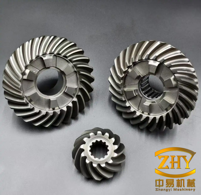
The face worm gear drive belongs to the family of screw gears, which are characterized by their spatial crossed-axis configuration and high sliding velocities. Unlike ordinary screw gears, face worm gear drives can achieve simultaneous meshing of multiple teeth, leading to high load capacity and smooth transmission. My work systematically examines the influence of geometric and manufacturing parameters on meshing performance, establishes a wear prediction model based on the Archard equation, and validates the theoretical findings through friction and wear tests as well as prototype experiments.
To begin, I establish a general mathematical model of the face worm gear drive based on differential geometry and spatial meshing theory. I define the reference coordinate systems and derive the coordinate transformation matrices. The worm tooth surface equations are obtained by considering the generating line of the worm. The meshing function, contact lines, and worm gear tooth surface equations are then derived. Furthermore, I deduce the first and second kind of limit functions, which are essential for evaluating the induced normal curvature and lubrication angle. These functions form the basis for analyzing the meshing performance of screw gears in face worm gear drives.
The coordinate systems employed in my model are as follows. Let $\Sigma_s(O_s: x_s, y_s, z_s)$ be the fixed coordinate system attached to the conical worm, and $\Sigma_m(O_m: x_m, y_m, z_m)$ be the moving coordinate system rigidly connected to the worm. The origins $O_s$ and $O_m$ coincide, and the $z_s$ and $z_m$ axes are collinear with the worm rotation axis. The worm rotation angle is $\varphi_1$. Similarly, $\Sigma_p(O_p: x_p, y_p, z_p)$ is the fixed coordinate system attached to the worm gear, and $\Sigma_n(O_n: x_n, y_n, z_n)$ is the moving coordinate system attached to the worm gear. The $z_p$ and $z_n$ axes are collinear with the worm gear axis. The center distance is $A$, the offset mounting distance of the worm is $Z_A$, and the thread length is $L_w$. The worm gear rotation angle is $\varphi_2$. The angular velocities of the worm and worm gear are $\omega_1$ and $\omega_2$, respectively, with the transmission ratio $i_{12} = \omega_1 / \omega_2 = \varphi_1 / \varphi_2$. The worm is right-handed.
The transformation matrices between these coordinate systems are given as follows:
$$\mathbf{M}_{ms} = \begin{bmatrix} \cos\varphi_1 & \sin\varphi_1 & 0 & 0 \\ -\sin\varphi_1 & \cos\varphi_1 & 0 & 0 \\ 0 & 0 & 1 & 0 \\ 0 & 0 & 0 & 1 \end{bmatrix}$$
$$\mathbf{M}_{sm} = \mathbf{M}_{ms}^{-1}$$
$$\mathbf{M}_{sp} = \begin{bmatrix} 1 & 0 & 0 & -A \\ 0 & 1 & 0 & 0 \\ 0 & 0 & 1 & A \\ 0 & 0 & 0 & 1 \end{bmatrix}$$
$$\mathbf{M}_{np} = \begin{bmatrix} \cos\varphi_2 & \sin\varphi_2 & 0 & 0 \\ -\sin\varphi_2 & \cos\varphi_2 & 0 & 0 \\ 0 & 0 & 1 & 0 \\ 0 & 0 & 0 & 1 \end{bmatrix}$$
$$\mathbf{M}_{pn} = \mathbf{M}_{np}^{-1}$$
$$\mathbf{M}_{nm} = \mathbf{M}_{np} \mathbf{M}_{ps} \mathbf{M}_{sm}$$
Expanding the last expression yields the complete transformation matrix from the worm coordinate system to the worm gear coordinate system, which involves the center distance $A$, the offset $E_A$, and the rotation angles. This matrix is essential for transforming the worm tooth surface into the worm gear coordinate system.
The generating line of the conical worm consists of two asymmetric straight lines, which produce the i-side and e-side tooth surfaces. In the axial section, the distance from any point on the generating line to the origin is denoted by $u$. The half-cone angle of the pitch cone is $\delta$. The profile angles of the i-side and e-side are $\alpha_i$ and $\alpha_e$, respectively, and the corresponding axial profile angles are $v_i$ and $v_e$, satisfying $v_i = \alpha_i – \delta$ and $v_e = -(\alpha_e + \delta)$.
The vector equation of the generating line for the i-side in the coordinate system $\Sigma_m$ is expressed as:
$$\mathbf{r}_i^{(m)} = x_i \mathbf{i}_m + y_i \mathbf{j}_m + z_i \mathbf{k}_m$$
$$x_i = u \cos\alpha_i$$
$$y_i = 0$$
$$z_i = u \sin\alpha_i$$
Similarly, for the e-side:
$$\mathbf{r}_e^{(m)} = x_e \mathbf{i}_m + y_e \mathbf{j}_m + z_e \mathbf{k}_m$$
$$x_e = u \cos\alpha_e$$
$$y_e = 0$$
$$z_e = -u \sin\alpha_e$$
The worm tooth surface is generated by the screw motion of these generating lines. The displacement of the tool during turning can be described by the axial screw parameter $p_x$ and the radial screw parameter $p_t$, with the relationship $p_t = p_x \tan\delta$. The transformation from the tool coordinate system $\Sigma_b$ to the worm coordinate system $\Sigma_w$ is given by:
$$\mathbf{M}_{wb} = \begin{bmatrix} \cos\varphi_u & -\sin\varphi_u & 0 & p_t \varphi_u \cos\varphi_u \\ \sin\varphi_u & \cos\varphi_u & 0 & p_t \varphi_u \sin\varphi_u \\ 0 & 0 & 1 & p_x \varphi_u \\ 0 & 0 & 0 & 1 \end{bmatrix}$$
where $\varphi_u$ is the screw motion angle. Applying this transformation to the generating lines yields the worm tooth surface equations. For the i-side, the components in $\Sigma_m$ are:
$$r_{ix} = (u \cos\alpha_i + p_t \varphi_u) \cos\varphi_u$$
$$r_{iy} = (u \cos\alpha_i + p_t \varphi_u) \sin\varphi_u$$
$$r_{iz} = p_x \varphi_u + u \sin\alpha_i$$
For the e-side:
$$r_{ex} = (u \cos\alpha_e + p_t \varphi_u) \cos\varphi_u$$
$$r_{ey} = (u \cos\alpha_e + p_t \varphi_u) \sin\varphi_u$$
$$r_{ez} = p_x \varphi_u – u \sin\alpha_e$$
The normal vectors to the worm tooth surfaces are obtained by taking the cross product of the partial derivatives with respect to $u$ and $\varphi_u$. For the i-side:
$$\mathbf{N}_i^{(m)} = \frac{\partial \mathbf{r}_i^{(m)}}{\partial u} \times \frac{\partial \mathbf{r}_i^{(m)}}{\partial \varphi_u}$$
Carrying out the differentiation yields the components $N_{ix}$, $N_{iy}$, and $N_{iz}$, which are functions of $u$, $\varphi_u$, and the geometric parameters. The unit normal vector is then $\mathbf{n}^{(m)} = \mathbf{N}^{(m)} / \sqrt{N_x^2 + N_y^2 + N_z^2}$. The same procedure applies to the e-side.
The meshing function in the coordinate system $\Sigma_m$ is defined as:
$$\Phi(u, \varphi_u) = \mathbf{n}^{(m)} \cdot \mathbf{v}^{(12)}$$
where $\mathbf{v}^{(12)}$ is the relative velocity between the worm and the worm gear at the meshing point. The relative velocity is computed from the angular velocities and position vectors:
$$\mathbf{v}^{(12)} = \boldsymbol{\omega}^{(1)} \times \mathbf{r}^{(m)} – \boldsymbol{\omega}^{(2)} \times \mathbf{r}^{(m)} – \boldsymbol{\omega}^{(2)} \times \mathbf{O}_m\mathbf{O}_n$$
In the coordinate system $\Sigma_m$, the angular velocity vectors are:
$$\boldsymbol{\omega}^{(1)} = \omega_1 \mathbf{k}_m$$
$$\boldsymbol{\omega}^{(2)} = \omega_2 (\sin\varphi_1 \mathbf{i}_m + \cos\varphi_1 \mathbf{j}_m)$$
The relative angular velocity is:
$$\boldsymbol{\omega}^{(12)} = \boldsymbol{\omega}^{(1)} – \boldsymbol{\omega}^{(2)} = -i_{12} \omega_2 \sin\varphi_1 \mathbf{i}_m + \omega_2 (1 – i_{12} \cos\varphi_1) \mathbf{j}_m + \omega_1 \mathbf{k}_m$$
The position vector of the origin of $\Sigma_n$ relative to $\Sigma_m$ is:
$$\mathbf{O}_m\mathbf{O}_n = -A \mathbf{i}_m + (A – E_A) \mathbf{j}_m + Z_A \mathbf{k}_m$$
Setting $\omega_1 = 1$ and $\omega_2 = i_{12}$, the relative velocity components become:
$$v_x^{(12)} = r_{iz} \cos\varphi_1 – r_{iy} i_{12} – E_A i_{12} \sin\varphi_1$$
$$v_y^{(12)} = r_{ix} i_{12} + r_{iz} \sin\varphi_1 + E_A i_{12} \cos\varphi_1$$
$$v_z^{(12)} = -i_{12} (r_{ix} \sin\varphi_1 + r_{iy} \cos\varphi_1) – A i_{12}$$
Substituting these into the meshing function gives the explicit expression for $\Phi$. The meshing equation is then $\Phi = 0$, which must be satisfied at all contact points.
The contact lines between the worm and worm gear tooth surfaces are obtained by solving the system of equations consisting of the worm tooth surface equation and the meshing equation. Transforming these contact lines into the coordinate system $\Sigma_n$ yields the worm gear tooth surface equation. The resulting equation for the i-side is:
$$\mathbf{r}_i^{(n)} = r_{ix}^{(n)} \mathbf{i}_n + r_{iy}^{(n)} \mathbf{j}_n + r_{iz}^{(n)} \mathbf{k}_n$$
where the components involve the transformation matrix $\mathbf{M}_{nm}$ and the worm surface coordinates. The e-side equation follows analogously. In these equations, there are four parameters: $\varphi_1$, $\varphi_2$, $\varphi_u$, and $u$. By using the transmission ratio relationship $i_{12} = \varphi_1 / \varphi_2$, the worm gear surface can be computed for a series of $\varphi_1$ values.
To evaluate the meshing performance, I derive the first and second kind of limit functions. The second kind of limit curve, also known as the meshing limit line, separates the meshing region from the non-meshing region on the worm gear tooth surface. It satisfies the conditions:
$$\Phi = 0$$
$$\Phi_t = 0$$
where $\Phi_t$ is the partial derivative of the meshing function with respect to time. The explicit expression for $\Phi_t$ is:
$$\Phi_t = \mathbf{n}^{(m)} \cdot \left[ (\boldsymbol{\omega}^{(1)} \times \boldsymbol{\omega}^{(2)}) \times \mathbf{r}^{(n)} – (\boldsymbol{\omega}^{(2)} \times \boldsymbol{\omega}^{(1)}) \times \mathbf{r}^{(m)} \right]$$
After substitution and simplification, the second kind of limit function becomes:
$$\Phi_t = n_x \left[ r_{iz} \sin\varphi_1 + (E_A – A) \omega_2 \right] + n_y \left[ r_{iz} \cos\varphi_1 – (E_A – A) \omega_2 \right] + n_z \left[ r_{ix} \sin\varphi_1 + r_{iy} \cos\varphi_1 \right]$$
The first kind of limit curve, also known as the undercut limit line, separates the working region from the interference region. It satisfies:
$$\Psi = \mathbf{a} \cdot \mathbf{v}^{(12)} + \Phi_t = 0$$
where the vector $\mathbf{a}$ is given by:
$$\mathbf{a} = \frac{1}{D} \left[ \Phi_u \left( \frac{\partial \mathbf{r}^{(m)}}{\partial u} \right) – \Phi \left( \frac{\partial \mathbf{r}^{(m)}}{\partial u} \right) \right] – \frac{1}{D} \left[ \Phi_{\varphi_u} \left( \frac{\partial \mathbf{r}^{(m)}}{\partial \varphi_u} \right) – \Phi \left( \frac{\partial \mathbf{r}^{(m)}}{\partial \varphi_u} \right) \right]$$
with $D = EG – F^2$, where $E$, $F$, and $G$ are the first fundamental quantities of the worm surface:
$$E = \left( \frac{\partial \mathbf{r}^{(m)}}{\partial u} \right)^2$$
$$F = \frac{\partial \mathbf{r}^{(m)}}{\partial u} \cdot \frac{\partial \mathbf{r}^{(m)}}{\partial \varphi_u}$$
$$G = \left( \frac{\partial \mathbf{r}^{(m)}}{\partial \varphi_u} \right)^2$$
The induced normal curvature $K_{\sigma}$ along the contact normal direction is then:
$$K_{\sigma} = \frac{\Psi}{\mathbf{a}^2}$$
The lubrication angle $\theta$ is defined as the angle between the contact line and the relative sliding velocity. It is computed as:
$$\theta = \arcsin\left( \frac{\mathbf{a} \cdot \mathbf{v}^{(12)}}{|\mathbf{a}| |\mathbf{v}^{(12)}|} \right)$$
A lubrication angle close to $90^\circ$ indicates favorable conditions for elastohydrodynamic lubrication. The relative entrainment velocity $v_n$ is the average of the velocities of the two surfaces at the contact point and is given by:
$$v_n = \frac{\mathbf{v}^{(\Sigma)} \cdot \mathbf{a}}{|\mathbf{a}|}$$
where $\mathbf{v}^{(\Sigma)}$ is the sum of the velocities of the worm and worm gear at the meshing point. These meshing performance functions are essential for evaluating the behavior of screw gears in face worm gear drives.
Based on my parametric study, I have summarized the influence of key design parameters on the meshing performance. The parameters considered include the center distance $A$, the offset mounting distance $Z_A$, the profile angle $v$, and the cone angle $\delta$. The results are presented in the following tables.
| Parameter | Symbol | Recommended Value | Effect on Induced Normal Curvature | Effect on Lubrication Angle | Effect on Entrainment Velocity |
|---|---|---|---|---|---|
| Center distance | $A$ | 94 mm | Decreases slightly with increase | Increases significantly | Increases slightly |
| Offset mounting distance | $Z_A$ | 65 mm | Increases with increase | Slight decrease | Slight increase |
| i-side profile angle | $v_i$ | 15° | Increases with increase | Increases with increase | Increases with increase |
| e-side profile angle | $v_e$ | 25° | Increases with increase | Increases with increase | Increases with increase |
| Cone half-angle | $\delta$ | 5° | Decreases with increase | Increases with increase | Increases with increase |
From the tables, I observe that the meshing performance is asymmetric between the i-side and e-side. The i-side generally exhibits a larger induced normal curvature and a slightly smaller lubrication angle compared to the e-side, indicating that the e-side has better load-carrying capacity while the i-side has better lubrication conditions. Along the tooth height direction, the induced normal curvature decreases from the tooth tip to the tooth root, while the lubrication angle and entrainment velocity increase. This implies that the tooth root region has better lubrication and lower wear, whereas the tooth tip is more prone to wear. The meshing entry region always has better lubrication than the meshing exit region.
Importantly, when the cone angle $\delta$ is reduced from 5° to 0°, the induced normal curvature increases by approximately 15%, and the lubrication angle decreases by only about 3%. This indicates that replacing the conical worm with a cylindrical worm in a face worm gear drive results in only a minor degradation of meshing performance, while greatly simplifying manufacturing. This finding supports the feasibility of using cylindrical worms in screw gears for face worm gear drives.
To facilitate the design and analysis of face worm gear drives, I developed a dedicated software tool using MATLAB and its APP Designer module. The software integrates functions for basic parameter calculation, geometric parameter calculation, tooth surface data generation, force calculation, and meshing performance analysis. The design flowchart is as follows: the user inputs the working conditions and material properties, the software calculates the center distance based on durability requirements, and then computes the geometric parameters using the reference point theory. The meshing performance is evaluated, and if it does not meet the requirements, the user can adjust the parameters. Once satisfactory, the tooth surface data points are computed and exported for solid modeling.
The software includes modules for:
- Basic parameter calculation
- Geometric parameter and installation dimension calculation
- Worm and worm gear tooth surface equation computation
- Induced normal curvature, lubrication angle, and relative entrainment velocity analysis
- Force calculation on the worm and worm gear
- Data saving and export
Using this software, I analyzed a typical case with an output power of 5 kW, an input speed of 1500 rpm, and a transmission ratio of 50. The calculated geometric parameters are summarized in the following table.
| Parameter | Symbol | Value |
|---|---|---|
| Module along pitch cone generatrix | $m_\delta$ | 3.73 mm |
| Center distance | $A$ | 94 mm |
| Transmission ratio | $i_{12}$ | 50 |
| Number of worm threads | $Z_1$ | 1 |
| Diameter coefficient | $q$ | 14 |
| Half-cone angle | $\delta$ | 5° |
| i-side profile angle | $v_i$ | 15° |
| e-side profile angle | $v_e$ | 25° |
| i-side axial screw parameter | $p_i$ | 1.8292 mm |
| e-side axial screw parameter | $p_e$ | 1.9517 mm |
| Worm small-end tip radius | $r_p$ | 26.11 mm |
| Worm thread length | $L_w$ | 68.62 mm |
| Nominal helix angle | $\beta$ | 85.9144° |
| Worm large-end tip radius | $r_{a1}$ | 32.11 mm |
| Offset mounting distance | $Z_A$ | 65 mm |
| Worm gear small-end tip radius | $R_{a1}$ | 110.37 mm |
| Worm gear large-end tip radius | $R_{a2}$ | 158.68 mm |
| Worm gear half-cone angle | $\delta_2$ | 83.3° |
For the strength analysis, I employed the Hertz contact theory to calculate the contact stress on the worm gear tooth surface. The maximum contact stress $\sigma_H$ is given by:
$$\sigma_H = \sqrt{\frac{K_A F_n}{\pi b} \frac{1}{\rho} \frac{1}{\frac{1 – u_1^2}{E_1} + \frac{1 – u_2^2}{E_2}}}$$
where $K_A$ is the application factor, $F_n$ is the normal force, $b$ is the effective contact width, $\rho$ is the equivalent curvature radius, and $E_1$, $E_2$, $u_1$, $u_2$ are the elastic moduli and Poisson’s ratios of the materials. The equivalent curvature radius is computed from the curvature radii of the worm and worm gear at the meshing point. For the i-side, the curvatures add, while for the e-side, they subtract. The contact stress results for different cone angles are presented in the following table, along with the finite element simulation results for validation.
| Worm gear surface | Numerical result (MPa) | FEM result (MPa) | Error (%) |
|---|---|---|---|
| i-side, $\delta = 5^\circ$ | 578.08 | 553.16 | 4.51 |
| e-side, $\delta = 5^\circ$ | 356.01 | 342.36 | 3.99 |
| i-side, $\delta = 0^\circ$ | 640.62 | 613.48 | 4.42 |
| e-side, $\delta = 0^\circ$ | 463.68 | 419.72 | 7.43 |
The results show that the e-side has a contact stress approximately 30% lower than the i-side, indicating better load-carrying capacity. When the cone angle is reduced from 5° to 0°, the contact stress increases by about 11%, which is consistent with the trend of the induced normal curvature. The finite element analysis confirms the accuracy of the analytical calculations, with errors within 10%.
For the wear analysis, I adopted the Archard wear equation, which relates the wear volume to the normal load, sliding distance, and material hardness:
$$V = \frac{K F_n s}{H}$$
where $V$ is the wear volume, $K$ is the dimensionless wear coefficient, $F_n$ is the normal load, $s$ is the sliding distance, and $H$ is the surface hardness. By introducing the contact area $A$, the wear depth $h$ can be expressed as:
$$h = \frac{V}{A} = k p s$$
where $k = K/H$ is the dimensional wear coefficient and $p$ is the contact pressure. For a meshing point, the wear depth after $n$ meshing cycles is:
$$h_n = h_{n-1} + k p \Delta s$$
The sliding distance $\Delta s$ per meshing cycle is approximated by:
$$\Delta s = 2 a_H \frac{|v_1 – v_2|}{v_2} = 2 a_H \frac{v_{12}}{v_2}$$
where $a_H$ is the Hertzian contact half-width, and $v_1$, $v_2$ are the surface velocities. The wear depth calculation is iterative: after each cycle, the tooth profile is updated to reflect the wear, and the contact pressure and half-width are recalculated. This coupled wear model allows me to predict the wear depth distribution on the worm gear tooth surface.
I calculated the wear depth for a contact line on the worm gear tooth surface under the following conditions: output torque $T_2 = 100$ N·m, elastic modulus $E = 2.11 \times 10^{11}$ Pa, Poisson’s ratio $u = 0.28$, wear coefficient $k = 5 \times 10^{-16}$ m²/N, worm speed $n_1 = 1500$ rpm, and $10^6$ meshing cycles. The results show that the wear depth is on the order of micrometers. Along the tooth height direction, the wear depth decreases from the tooth tip to the tooth root, which is consistent with the lubrication analysis: the tooth tip has poorer lubrication and thus higher wear. The e-side exhibits greater wear depth than the i-side, confirming the inferior lubrication conditions on the e-side. Increasing the profile angle and the cone angle reduces the wear depth, as these changes improve the lubrication angle and reduce the induced normal curvature.
To validate the wear model, I designed and conducted pin-on-disk friction and wear experiments. The pin and disk specimens were made of 42CrMo steel, nitrided to a hardness of 55-58 HRC, and polished. The pin had a spherical end with a radius equal to the induced normal curvature radius at the meshing point. The disk was rotated at a controlled speed, and a normal load of 150 N was applied. The lubrication angle was varied from 0° to 90° by orienting the pin relative to the sliding direction. The tests were conducted under oil lubrication with a 460# worm gear oil. The friction coefficient and wear depth were measured.
The experimental results are summarized in the following table. The friction coefficient decreases as the lubrication angle increases, and the wear depth also decreases. For a given lubrication angle, a larger induced normal curvature radius (i.e., smaller curvature) results in a smaller friction coefficient and wear depth. These trends are consistent with the theoretical predictions and confirm the importance of lubrication angle and curvature in screw gears.
| Lubrication angle (°) | Wear depth, $R=29$ mm (µm) | Wear depth, $R=32$ mm (µm) | Wear depth, $R=35$ mm (µm) | Wear depth, $R=40$ mm (µm) |
|---|---|---|---|---|
| 0 | 14.5 | 13.2 | 12.1 | 11.3 |
| 22.5 | 10.8 | 9.9 | 9.2 | 8.6 |
| 45 | 7.6 | 7.1 | 6.7 | 6.3 |
| 67.5 | 5.9 | 5.5 | 5.2 | 4.9 |
| 90 | 4.8 | 4.5 | 4.3 | 4.1 |
Encouraged by these results, I proceeded to design and manufacture a prototype of a face worm gear reducer. The prototype employs a double-support straddle mounting for both the worm and worm gear shafts. The worm shaft is supported by a combination of deep groove ball bearings and double-row tapered roller bearings, while the worm gear shaft uses similar bearings. The stiffness of the worm was checked under the allowable torque to ensure that the maximum deflection does not exceed the permissible value. The allowable torque was calculated using the following formula:
$$[T_2] = \frac{K_m L_\Sigma r_{w2}}{K_w k_N^{(12)}}$$
where $K_m$ is the allowable wear coefficient, $L_\Sigma$ is the contact line length, $r_{w2}$ is the working radius of the worm gear, $K_w$ is the working condition factor, and $k_N^{(12)}$ is the induced principal curvature at the midpoint of the tooth surface. The calculated allowable torque is 1610.6 N·m. The maximum deflection of the worm was found to be 0.0137 mm, which is within the allowable range of 0.01865–0.0373 mm. The theoretical meshing efficiency was estimated using the formula:
$$\eta = \frac{\cos\alpha_{mn} + u \tan\beta_{m1}}{\cos\alpha_{mn} + u \tan\beta_{m2}}$$
where $\alpha_{mn}$ is the normal profile angle, $\beta_{m1}$ and $\beta_{m2}$ are the helix angles at the midpoint of the worm and worm gear, and $u$ is the friction coefficient. The calculated efficiencies are 76.8% for the i-side and 79.6% for the e-side. Accounting for bearing losses and oil splashing, the overall efficiencies are approximately 74.5% and 77.2%.
The manufacturing processes for the key components are as follows. The worm was turned, ground on a four-axis CNC machine, nitrided, and polished. The conical worm gear was machined on a five-axis machining center, nitrided, and polished. The cylindrical worm gear was hobbed using a double-lead cylindrical hob. The machining accuracy of the worm gear tooth surface was inspected using a coordinate measuring machine. The average deviations were 0.0329 mm for the i-side and 0.034 mm for the e-side, meeting the accuracy requirements.
The experimental setup for transmission performance testing consisted of a servo motor, input torque sensor, prototype reducer, output torque sensor, speed increaser, and magnetic powder brake. The input speed was set to 1500 rpm, and the output load was increased in steps of 100 N·m. The transmission efficiency was calculated from the ratio of output power to input power. The contact pattern was checked by applying red lead powder to the worm gear teeth and observing the contact areas after running. The results showed that the i-side had six pairs of teeth in contact, while the e-side had five pairs, indicating good contact conditions.
The transmission efficiency and load capacity of the face worm gear reducer were compared with a conventional cylindrical worm reducer of similar parameters. The results are presented in the following table.
| Reducer type | Efficiency (%) | Load capacity (N·m) |
|---|---|---|
| Cylindrical worm reducer (forward) | 46 | 360 |
| Cylindrical worm reducer (reverse) | 46 | 360 |
| Face worm gear drive, $\delta=5^\circ$, i-side | 73.9 | 1100 |
| Face worm gear drive, $\delta=5^\circ$, e-side | 74.3 | 1400 |
| Face worm gear drive, $\delta=0^\circ$, i-side | 69.3 | 1000 |
| Face worm gear drive, $\delta=0^\circ$, e-side | 71.0 | 1200 |
The face worm gear drive demonstrates a transmission efficiency approximately 1.6 times that of the conventional cylindrical worm reducer and a load capacity up to 3.8 times higher. The e-side consistently outperforms the i-side in both efficiency and load capacity, which is consistent with the meshing performance analysis. When the cone angle is reduced from 5° to 0°, the efficiency decreases by 6.6% for the i-side and 4.6% for the e-side, while the load capacity decreases by 10% and 16%, respectively. These results confirm that the cylindrical worm version of the face worm gear drive retains most of the advantages of the conical worm version.
After the experiments, I inspected the tooth surface wear on both the worm and worm gear. The wear pattern on the worm gear showed that the tooth tip region had more pronounced wear than the tooth root region, and the e-side had greater wear than the i-side. The meshing entry region exhibited less wear than the meshing exit region. These observations are in good agreement with the wear model predictions and the lubrication analysis. The experimental results thus provide strong validation for my theoretical and numerical investigations.
In conclusion, my research on face worm gear drives as a type of screw gears has led to the following key findings:
- The general mathematical model and meshing performance functions provide a solid theoretical foundation for analyzing screw gears in face worm gear drives.
- The meshing performance is asymmetric between the i-side and e-side, with the e-side exhibiting better load capacity and the i-side exhibiting better lubrication. The meshing entry region has better lubrication than the exit region.
- Replacing the conical worm with a cylindrical worm in a face worm gear drive results in only minor degradation of meshing performance, making it a viable solution for improving manufacturability.
- The wear model based on the Archard equation accurately predicts the wear depth distribution, and the friction and wear experiments confirm the influence of lubrication angle and curvature radius.
- The prototype experiments demonstrate that the face worm gear drive significantly outperforms conventional cylindrical worm reducers in terms of efficiency and load capacity, validating its potential for high-rigidity robotic joint applications.
- The developed design and analysis software greatly improves the efficiency of parameter design and performance optimization for screw gears in face worm gear drives.
Future work should focus on optimizing the basic parameters using multi-objective optimization techniques and further refining the wear model by coupling thermal effects and lubrication characteristics. These efforts will further promote the application of face worm gear drives in industrial robotics and other demanding fields.