
I have focused my research on the problem of improving the efficiency, programmability, and stability of gear hobbing when it is performed on a mill-turn machining center rather than on a dedicated hobbing machine. Gear hobbing remains one of the most widely used methods for producing cylindrical gears because it offers high productivity, good contour accuracy, and broad applicability to different gear types. However, when gear hobbing is transferred to a multi-axis mill-turn platform, several difficulties appear: the numerical control program is usually written for one specific gear, the machining parameters are selected mainly by operator experience, and there is no reliable pre-verification method before the real cut. These issues reduce the reuse rate of the program, increase programming time, and make the process sensitive to parameter mismatch. In my work, I therefore treat gear hobbing as an integrated problem that includes kinematic modeling, parametric program generation, customized human-machine interface development, virtual simulation, and multi-objective parameter optimization. The platform I use is a BHR700V mill-turn machining center. I build the motion model of gear hobbing, establish the mapping between gear parameters and numerical control instructions, generate the part program automatically from macro variables, verify the program in a virtual dual-channel environment, and finally optimize the cutting speed, axial feed, and radial depth of cut by using an improved NSGA-II algorithm. The objective is to obtain a gear hobbing process that is reusable, verifiable, and balanced between machining time and tool wear.
Introduction. Gears are core transmission components in modern machinery. Their accuracy, surface integrity, and consistency directly affect load capacity, transmission efficiency, noise, and service life. Among the available manufacturing methods, gear hobbing is especially important because it uses a continuous generating motion, it can cut spur gears, helical gears, splines, and worm wheels, and it is suitable for automatic control. In a traditional gear hobbing machine, the motion relationship between the hob and the workpiece is guaranteed by a mechanical transmission chain. In a mill-turn machining center, the same relationship must be established electronically by the numerical control system. This change brings flexibility but also introduces new requirements: the electronic gear ratio must be accurate, the feed axes must be coordinated, and the program must be able to adapt to different gear specifications without being rewritten from scratch. I observed that many existing gear hobbing programs are fixed-code programs. When the module, number of teeth, helix angle, or face width changes, the programmer must edit many lines manually. This is slow, error-prone, and unsuitable for small-batch, multi-variety production. Moreover, the machining parameters are often chosen from a handbook or from experience, and the trade-off between machining time and tool wear is rarely quantified. I therefore decided to develop a parametric programming method and a multi-objective optimization method for gear hobbing on a mill-turn center.
Kinematic analysis of gear hobbing. In gear hobbing, the hob behaves like a rack with helical cutting edges. The workpiece and the hob maintain a strict meshing relationship. As the hob rotates, the workpiece rotates at a proportional speed, and the hob also moves along the axis of the workpiece. The tooth profile is generated by the envelope of the cutting edges over time. The three basic motions are the main motion, the indexing motion, and the feed motion. The main motion is produced by the hob spindle. Its cutting speed is
$$ v_c = \frac{\pi D n_c}{1000} $$
where \(v_c\) is the cutting speed in m/min, \(D\) is the hob outside diameter in mm, and \(n_c\) is the hob rotational speed in r/min. The main motion determines the cutting temperature, the tool wear rate, and the material removal efficiency. The indexing motion is the most critical motion in gear hobbing because it guarantees the correct number of teeth. The relationship between the hob speed and the workpiece speed is
$$ \frac{n_w}{n_c} = \frac{z_c}{z_w} $$
where \(n_w\) is the workpiece rotational speed, \(z_c\) is the number of hob starts, and \(z_w\) is the number of gear teeth. This ratio is the foundation of the electronic gearbox in a mill-turn center. The feed motion consists of axial feed and radial feed. The axial feed moves the hob along the face width so that the full tooth width can be cut. The radial feed moves the hob toward the workpiece so that the tooth depth is reached gradually. The feed speed is
$$ v_f = f_a n_c $$
where \(f_a\) is the axial feed per hob revolution in mm/rev. The axial feed has a strong influence on tooth flank quality, chip load, and machining time. If the feed is too high, the cutting force increases and the tool wear becomes severe. If the feed is too low, the machining time becomes unnecessarily long. Therefore, the selection of feed and speed must be treated as a coordinated decision rather than an isolated choice.
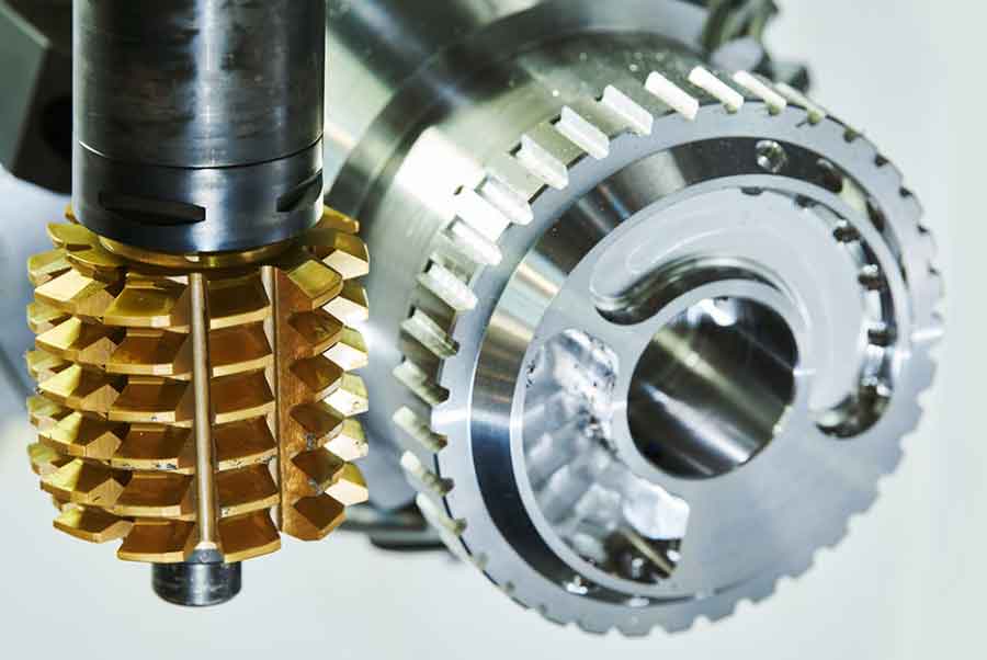
Tooth profile generation and error sources. The tooth profile in gear hobbing is not copied from the tool shape. It is generated by the relative motion between the hob and the workpiece. The involute profile is produced when a straight line rolls without slipping on a base circle. In gear hobbing, the hob is equivalent to a rack cutter, and the workpiece is equivalent to the gear that meshes with that rack. The cutting edges create a family of instantaneous envelope surfaces, and the continuous superposition of these surfaces forms the final involute tooth. The process can be divided into an entry stage, a steady cutting stage, and an exit stage. In the entry stage, only a few teeth participate in cutting. In the steady stage, multiple teeth cut simultaneously, and the load becomes more uniform. In the exit stage, the cutting load decreases until the tooth is complete. This behavior makes gear hobbing a multi-edge intermittent cutting process with periodic load fluctuation. The main error sources in gear hobbing include motion synchronization errors, tool manufacturing and installation errors, cutting-force-induced deformation, vibration and stability errors, and tool wear. Motion synchronization error is especially important because any deviation between the hob rotation and the workpiece rotation directly changes the tooth spacing and the tooth profile. Tool runout and axial movement also accumulate into profile error. Cutting force is generated by plastic deformation, friction, and chip formation, and it can deform the machine structure, the tool, and the workpiece. Vibration appears because the cutting force fluctuates periodically as the teeth enter and leave the cut. Tool wear changes the cutting edge geometry and therefore affects the tooth profile and surface quality. For these reasons, the machining parameters must be selected not only for productivity but also for stability and tool life.
Mill-turn platform and axis configuration. The BHR700V mill-turn machining center has a horizontal opposed dual-spindle layout. The upper turret has a rotary B axis, and the lower turret is a horizontal power turret. The machine uses high-speed turning and milling motorized spindles, roller linear guideways, and a chain tool magazine. It supports five-axis simultaneous machining, turning and milling integration, and high-speed high-precision operation. The machine has two rotary axes, C1 and C2, and several linear axes. The axis functions are summarized in Table 1.
| Axis | Function |
|---|---|
| X1 | Upper turret vertical motion |
| X2 | Lower turret inclined motion |
| Z1 | Milling spindle horizontal motion |
| Z2 | Turning spindle horizontal motion |
| W | Sub-spindle horizontal motion |
| Y | Upper turret fore-aft motion |
| B | Milling spindle swing |
| C1 | Rotary axis 1 |
| C2 | Rotary axis 2 |
For gear hobbing on this machine, the essential kinematic requirement is that the hob spindle and the workpiece spindle maintain an accurate speed ratio. The numerical control system supports electronic gearbox functions, so the ratio can be set and changed by program. The axial feed is provided by a linear axis, and the radial feed is provided by another linear axis. In this way, the basic motion relation of gear hobbing is reproduced on a mill-turn platform. Compared with a dedicated gear hobbing machine, the mill-turn platform is more flexible, but it relies more heavily on the numerical control synchronization and on the correctness of the parameter matching. This is exactly why parametric programming and parameter optimization are necessary. Without them, the gear hobbing process on a mill-turn center would remain a manual, experience-dependent operation.
Parametric programming principles. Parametric programming means that fixed numerical values in the part program are replaced by variables, and the relationships among these variables are described by mathematical expressions. In the Siemens ONE control system, variables can be defined, calculated, compared, and used in conditional statements. For gear hobbing, the gear module, number of teeth, pressure angle, helix angle, face width, and tooth depth determine the geometry of the workpiece. The spindle speed, axial feed, and radial depth of cut determine the cutting condition. By establishing the functional relationships among these parameters, the program can calculate the required motion automatically. When the gear specification changes, the operator only needs to enter a new set of parameters, and the program regenerates the tool path and the numerical control instructions. This reduces programming time and avoids manual editing errors. I developed the parametric gear hobbing program in a modular way. The modules include a human-machine interface input module, a tool setting module, a calculation module, a synchronization module, a cycle machining module, and an end-of-program reset module.
Feature parameter extraction. To build a parametric program for gear hobbing, I first identified the parameters that have clear physical meaning and independent adjustability. The gear structure parameters determine the workpiece geometry and the generating motion. The module determines the pitch diameter and tooth height. The number of teeth determines the indexing ratio. The pressure angle determines the involute shape and the hob selection. The helix angle affects the relationship between axial feed and workpiece rotation. The face width determines the axial stroke. The tooth depth determines the radial depth of cut. These parameters are independent input variables for different gear specifications. The machining parameters influence the cutting load and the stability but do not change the theoretical gear geometry. They include radial depth of cut, axial feed, spindle speed, and feed speed. I summarized the main parametric variables in Table 2.
| Category | Parameter | Symbol |
|---|---|---|
| Gear structure | Module | \(m\) |
| Gear structure | Number of teeth | \(z\) |
| Gear structure | Pressure angle | \(\alpha\) |
| Gear structure | Helix angle | \(\beta\) |
| Gear structure | Face width | \(B\) |
| Gear structure | Tooth depth | \(h\) |
| Machining | Radial depth of cut | \(a_p\) |
| Machining | Axial feed | \(f_a\) |
| Machining | Spindle speed | \(n\) |
| Machining | Feed speed | \(v_f\) |
Tool path selection for gear hobbing. The tool path in gear hobbing determines how the hob approaches the workpiece, how the depth is reached, and how the face width is traversed. Two common strategies are the radial-axial feed method and the axial reciprocating feed method. In the radial-axial method, the hob first feeds radially to the full tooth depth and then moves axially across the face width. This method is simple and efficient, but the radial engagement is large, the cutting force is high, and the tool wear is concentrated. It is suitable for stable conditions and for small modules. In the axial reciprocating method, the hob feeds radially by a small amount, then moves axially across the face width, then feeds radially again, and repeats this sequence until the full tooth depth is reached. This method reduces the single-pass cutting load, improves stability, and distributes the wear more evenly. Although the total machining time may be slightly longer, the process is more stable and more suitable for a mill-turn platform where the gear hobbing parameters may vary from one workpiece to another. I selected the axial reciprocating feed method as the main tool path for the parametric gear hobbing program. This choice improves the robustness of the program and reduces the risk caused by parameter changes.
Program structure and macro control. The gear hobbing program is built around macro variables and structured control statements. The first step is to set the absolute programming mode, the workpiece coordinate system, the metric unit, and the feed unit. The second step is to start the workpiece spindle and establish the electronic gearbox between the hob axis and the workpiece axis. The third step is to calculate the number of radial passes from the tooth depth and the radial depth of cut. The fourth step is to control the radial feed in a loop. The fifth step is to calculate the number of axial passes from the face width and the axial feed. The sixth step is to control the axial reciprocating motion in a loop while the hob and the workpiece remain synchronized. The seventh step is to perform the final radial pass to the full tooth depth and the final axial pass across the full face width. The eighth step is to cancel the synchronization, retract the tool to a safe position, stop the spindle, turn off the coolant, and reset the program. This structure makes the gear hobbing program general and reusable.
In the synchronization module, the electronic gear ratio is calculated from the number of gear teeth and the number of hob starts:
$$ \text{ratio} = \frac{N_{\text{teeth}}}{Z_{\text{cutter}}} $$
The control system then defines the gearbox with the workpiece axis as the master and the hob axis as the slave. The synchronization is activated before cutting and deactivated after cutting. A simplified macro sequence is shown below in concept:
G90 G54
A0 C0
EGBDEF(C, A, ratio)
EGBON
S = n_c M3
...
EGBOFF
The calculation module converts continuous physical quantities into integer loop counts. For example, the number of radial passes is obtained by dividing the tooth depth by the radial depth of cut, and the result is then converted into an integer for loop control. The axial passes are calculated in the same way. This is important because the numerical control system must execute a finite number of passes, while the physical depth and width are continuous variables. The loop structure makes the gear hobbing program adapt automatically to different tooth depths and face widths.
Customized human-machine interface. A parametric program is powerful, but it still requires the operator to understand the variables and the program logic. To make the gear hobbing process more practical, I developed a customized human-machine interface on the Siemens ONE platform. The interface is built with a screen definition file and a global variable file. The screen definition file creates buttons, text labels, input fields, and help images. The global variable file defines the variables that are shared between the interface and the numerical control program. When the operator enters a value in an input field, the value is written into the corresponding global variable. The gear hobbing program then reads the global variable and uses it in the calculation and motion control. In this way, the interface becomes a parameter input station for gear hobbing, and the numerical control program becomes a reusable engine that generates the machining process.
The interface is organized by parameter category. Gear parameters such as module, number of teeth, pressure angle, helix angle, face width, and tooth depth are placed in one area. Machining parameters such as radial depth of cut, spindle speed, and feed rate are placed in another area. Tool setting coordinates are placed in a third area. When an input field receives focus, the interface can display a help image that explains the physical meaning of the parameter. This reduces the chance of wrong input and makes the interface suitable for operators who are not programming experts. The global variables I defined are listed in Table 3.
| Variable | Data type |
|---|---|
| Module | REAL |
| Number of teeth | INT |
| Pressure angle | REAL |
| Helix angle | REAL |
| Tool setting X0 | REAL |
| Tool setting Y0 | REAL |
| Tool setting Z0 | REAL |
| Tooth depth | REAL |
| Face width | REAL |
| Radial depth of cut | REAL |
| Spindle speed | REAL |
| Feed rate | REAL |
| Addendum allowance | REAL |
| Flank allowance | REAL |
After the interface and the variable binding were completed, I tested the gear hobbing function in a virtual numerical control environment. I created a machine model that matches the axis configuration of the mill-turn center, and I set the control system type, the axis structure, and the spindle configuration. The interface was then laid out with consistent fonts, sizes, and colors. During the test, I entered a set of gear parameters and observed whether the variables were transferred correctly to the program. The results showed that the interface responded normally, the help images were displayed correctly, and the program was generated and executed without alarm or logical conflict. The tool path and the spindle synchronization matched the expected gear hobbing motion. This confirmed that the parametric program and the customized interface can support practical gear hobbing on the mill-turn platform.
Virtual machine modeling. To verify the gear hobbing program before real machining, I built a virtual simulation environment. The machine structure is complex, so I divided it into functional modules: bed, spindle, X-axis guideway, Y-axis guideway, Z-axis guideway, turret, tool magazine, tailstock, and chucks. I modeled each module in UG, assembled them according to the actual machine layout, and exported the components in STL format for VERICUT. The assembly used the machine origin as the reference, so the relative positions of the components were preserved after import. The virtual machine includes the main structural components and the motion axes. The base node contains the linear and rotary axes, and each axis carries the corresponding geometric model. The component tree reflects the actual motion topology of the mill-turn center.
The axis topology is divided into several branches. One branch starts from the bed and carries the Z1 axis, the Y axis, and the X1 axis, and the milling spindle with the B axis is mounted at the end of this chain. Another branch carries the C1 rotary axis and the chuck for the main workpiece spindle. A third branch carries the Z2 and X2 axes and the lower turret. A fourth branch carries the W axis and the C2 rotary axis with the sub-chuck. This structure allows the virtual machine to reproduce both turning and milling motions. For gear hobbing, the hob is mounted on the milling spindle, and the workpiece is mounted on the main spindle. The electronic gearbox relation is realized through the control system and the synchronized motion of the two rotary axes.
Dual-channel configuration. The mill-turn center uses a dual-channel numerical control system. Each channel has its own interpolation unit, variables, and program execution. The two channels can run independently or synchronously. In the virtual environment, I configured the milling channel and the turning channel separately. The milling channel includes the milling spindle, the X1 axis, the Y axis, the Z1 axis, and the B axis. The turning channel includes the Z2 axis and the X2 axis. The shared axes C1 and C2 are assigned to both channels. For gear hobbing, the synchronization between the hob spindle and the workpiece spindle is the key function. I therefore loaded two programs in the synchronous program configuration, one for each channel, and specified the corresponding subsystem IDs. When synchronization is not required, the second program can be disabled. This dual-channel setup makes the virtual simulation consistent with the real machine behavior.
Tool and workpiece setup. I imported the hob model into the VERICUT tool manager. The hob is not a standard tool type in the library, so I used the external model import function. The clamping direction and the clamping point were set to the origin of the hob coordinate system. The workpiece blank was modeled according to the gear dimensions, and the fixture was positioned according to the actual clamping scheme. The program zero was defined by the G-code offset. Because the machine has two channels and two work areas, I used the work offset method rather than the single program zero method. The offset was assigned to the milling and turning subsystems, and the registers were set to 54 and 55. The tool was positioned relative to the coordinate origin of each channel. This ensured that the gear hobbing program could be executed in the correct coordinate frame.
Simulation of gear hobbing. After the virtual machine, the tool, the workpiece, and the program were configured, I ran the gear hobbing simulation. The simulation displayed the relative motion between the hob and the workpiece. The hob rotated at the commanded speed, the workpiece rotated according to the electronic gear ratio, and the axial feed moved the hob along the face width. The radial feed was applied in steps until the full tooth depth was reached. The simulation detected no collision, no interference, and no overtravel. The tool path was stable, and the tooth profile was generated correctly. I then used the automatic comparison function to compare the simulated gear model with the design model. The comparison showed that the tooth profile matched the design within a small deviation, and the overall structure was correct. This verified the logic of the parametric gear hobbing program and the feasibility of the process on the mill-turn center.
Multi-objective optimization problem. The quality of gear hobbing depends strongly on the cutting parameters. The cutting speed, the axial feed, and the radial depth of cut influence both the machining time and the tool wear. Increasing the cutting speed or the feed reduces the machining time but accelerates tool wear. Decreasing them prolongs tool life but increases the machining time. Therefore, the parameter selection for gear hobbing is a multi-objective optimization problem. I selected the cutting speed \(V\), the axial feed \(f_a\), and the radial depth of cut \(a_e\) as the optimization variables:
$$ X = [V, f_a, a_e] $$
The first objective is the machining time. The total stroke of the gear hobbing process is the sum of the tooth depth, the approach and overrun, and the face width:
$$ L = h + l_1 + l_2 + b $$
where \(h\) is the tooth depth, \(l_1\) and \(l_2\) are the approach and overrun, and \(b\) is the face width. The machining time is
$$ T(X) = \frac{L}{f_a n} $$
where \(n\) is the hob rotational speed. Since
$$ n = \frac{1000 V}{\pi D} $$
the machining time model becomes
$$ T(X) = \frac{L \pi D}{1000 V f_a} $$
The second objective is the tool wear. I used a power-law model to describe the relative wear trend:
$$ W = k V^{\alpha} f_a^{\beta} a_e^{\gamma} $$
where \(k\) is a coefficient, and \(\alpha\), \(\beta\), and \(\gamma\) are exponents related to the tool and workpiece materials. The model is not intended to predict the absolute wear volume but to represent the relative influence of the cutting parameters. The objective functions are therefore minimized simultaneously:
$$ \min f_1(X) = T(X) $$
$$ \min f_2(X) = W(X) $$
Constraints and process conditions. The optimization must respect the machine capability and the process requirements. The gear hobbing process considered here is a roughing operation. The workpiece material is 45 steel, the module is 5.35, the face width is 21 mm, the tooth depth is 13.85 mm, the hob material is high-speed steel, and the hob pitch diameter is 93.3 mm. The surface roughness after roughing is allowed to be in the range of Ra 6.3 to 12.5 micrometers. The constraints on the optimization variables are
$$ 15 \le V \le 30 \ \text{m/min} $$
$$ 1.1 \le f_a \le 2.1 \ \text{mm/rev} $$
$$ 0.5 \le a_e \le 0.6 \ \text{mm} $$
These ranges ensure that the roughing operation can remove the required material without overloading the machine or producing unacceptable tool wear. They also provide a stable basis for the subsequent finishing operation.
Selection of the optimization method. Several multi-objective methods are available. The weighted sum method is simple but cannot find solutions on a non-convex Pareto front, and it is sensitive to the weights. Goal programming is suitable when one objective has priority over the other, but it does not provide a balanced set of alternatives. Pareto-based evolutionary algorithms, such as NSGA-II, NSGA-III, and SPEA2, directly search for the Pareto front and can produce a set of compromise solutions. For a two-objective gear hobbing problem with nonlinear objectives and continuous variables, NSGA-II is a suitable choice. It uses non-dominated sorting and crowding distance to maintain convergence and diversity. I therefore selected NSGA-II and improved its mutation operator to better balance global exploration and local exploitation.
NSGA-II procedure for gear hobbing. The algorithm starts by initializing a population of candidate parameter sets within the allowed ranges. Each individual represents a combination of cutting speed, axial feed, and radial depth of cut. The objective functions are evaluated for each individual. The population is then sorted into non-dominated fronts. The first front contains the individuals that are not dominated by any other individual. The second front contains the individuals that become non-dominated after the first front is removed. This process continues until all individuals are assigned to a front. Crowding distance is calculated within each front to measure how close an individual is to its neighbors. For a two-objective problem, the crowding distance of the \(i\)-th individual is
$$ d_i = \sum_{m=1}^{2} \frac{|f_m(i+1) – f_m(i-1)|}{f_m^{\max} – f_m^{\min}} $$
Individuals with larger crowding distance are preferred because they lie in sparser regions of the objective space. The selection operator uses tournament selection based on non-dominated rank and crowding distance. The crossover operator uses simulated binary crossover, which recombines the variables of two parents to produce two children. The mutation operator applies a small random perturbation to the variables. The parent and child populations are then merged, and the combined population is sorted again. The next generation is filled front by front, and within the last front, the individuals with the largest crowding distance are selected until the population size is restored. This elitist strategy preserves good solutions and maintains diversity.
Improved adaptive mutation. In the standard NSGA-II, the mutation probability is fixed. This can cause insufficient diversity in the early stage and unstable convergence in the late stage. I introduced an adaptive mutation probability that decreases with the generation number:
$$ p_m(t) = p_{m0} \left(1 – \frac{t}{T_{\max}}\right) $$
where \(p_{m0}\) is the initial mutation probability, \(t\) is the current generation, and \(T_{\max}\) is the maximum generation. In the early stage, the mutation probability is relatively high, which increases population diversity and expands the search range. In the late stage, the mutation probability decreases, which stabilizes the search near the Pareto front. This improves the balance between exploration and exploitation. The termination criterion is the maximum generation. Based on preliminary tests, the Pareto front changes little after 150 generations, so I set \(T_{\max} = 150\).
MATLAB implementation and Pareto results. I implemented the improved NSGA-II in MATLAB 2021b. The algorithm was run for 150 generations. The resulting Pareto front is shown in Table 4. The solutions are distributed along a trade-off curve. Moving from the first solution to the last solution, the machining time decreases and the tool wear increases. This confirms the expected conflict between productivity and tool life in gear hobbing. The solutions are not clustered in a single region, which indicates that the diversity preservation mechanism is working.
| No. | \(V\) (m/min) | \(f_a\) (mm/rev) | \(a_e\) (mm) | \(T\) (min) | \(W\) |
|---|---|---|---|---|---|
| 1 | 15.000 | 1.1000 | 0.50000 | 0.97437 | 121.41 |
| 2 | 15.294 | 1.1799 | 0.50029 | 0.89094 | 133.58 |
| 3 | 15.015 | 1.2970 | 0.50074 | 0.82554 | 139.00 |
| 4 | 15.772 | 1.3561 | 0.50626 | 0.75165 | 160.70 |
| 5 | 16.167 | 1.4524 | 0.51207 | 0.68470 | 180.40 |
| 6 | 16.259 | 1.7357 | 0.51106 | 0.56971 | 210.00 |
| 7 | 16.272 | 1.9596 | 0.50747 | 0.50421 | 230.15 |
| 8 | 18.622 | 1.8617 | 0.50244 | 0.46374 | 286.45 |
| 9 | 18.745 | 2.0484 | 0.50293 | 0.41871 | 313.62 |
| 10 | 22.424 | 2.0530 | 0.50271 | 0.34923 | 449.42 |
| 11 | 23.378 | 2.0599 | 0.51036 | 0.33386 | 497.23 |
| 12 | 24.147 | 2.0690 | 0.52699 | 0.32180 | 549.72 |
| 13 | 25.115 | 2.0380 | 0.57207 | 0.31410 | 637.82 |
| 14 | 28.438 | 2.0662 | 0.51036 | 0.27361 | 737.59 |
| 15 | 29.553 | 2.0778 | 0.50782 | 0.26182 | 796.17 |
| 16 | 29.910 | 2.0763 | 0.53523 | 0.25888 | 859.01 |
| 17 | 29.856 | 2.0872 | 0.58215 | 0.25799 | 934.89 |
| 18 | 29.999 | 2.0984 | 0.57813 | 0.25539 | 941.36 |
| 19 | 30.000 | 2.0995 | 0.65374 | 0.25526 | 1065.0 |
Decision-making from the Pareto set. The Pareto set contains many non-dominated solutions. To select one parameter combination for practical use, I applied a normalized weighted scoring method. The machining time and the tool wear were normalized separately. Because both objectives are to be minimized, the normalized score for the machining time is
$$ T_i^* = \frac{T_{\max} – T_i}{T_{\max} – T_{\min}} $$
and the normalized score for the tool wear is
$$ W_i^* = \frac{W_{\max} – W_i}{W_{\max} – W_{\min}} $$
The overall score is then
$$ S_i = 0.5 T_i^* + 0.5 W_i^* $$
The solution with the largest \(S_i\) is chosen as the compromise solution when machining efficiency and tool life are considered equally important. In the field, I found that the operators apply a spindle speed override of 0.8 and an axial feed override of 0.02 to match the actual cutting condition. To make the model consistent with the real process, I introduced these correction factors:
$$ V_{\text{real}} = 0.8 V $$
$$ f_{a,\text{real}} = 0.02 f_a $$
I then recalculated the machining time and the tool wear for each Pareto solution. The results are shown in Table 5. The ninth solution has the highest score, so it was selected as the compromise optimum. Its parameters are \(V = 18.745\) m/min, \(f_a = 2.0484\) mm/rev, and \(a_e = 0.50293\) mm. The cutting speed is in the middle-upper range, which avoids both the low efficiency of a very low speed and the high load of a very high speed. The axial feed is close to the upper bound, which improves productivity while keeping the cutting force fluctuation acceptable. The radial depth of cut is near the middle of its range, which supports stable tooth depth control and consistent quality.
| No. | \(V\) (m/min) | \(f_a\) (mm/rev) | \(a_e\) (mm) | \(V_{\text{real}}\) (m/min) | \(f_{a,\text{real}}\) (mm/rev) | \(T\) (min) | \(W\) | \(T_i^*\) | \(W_i^*\) | \(S_i\) |
|---|---|---|---|---|---|---|---|---|---|---|
| 1 | 15.000 | 1.1000 | 0.50000 | 12.000 | 0.02200 | 60.90 | 121.41 | 0.0000 | 1.0000 | 0.5000 |
| 2 | 15.294 | 1.1799 | 0.50029 | 12.235 | 0.02360 | 55.68 | 133.58 | 0.1161 | 0.9879 | 0.5520 |
| 3 | 15.015 | 1.2970 | 0.50074 | 12.012 | 0.02594 | 51.60 | 139.00 | 0.2069 | 0.9828 | 0.5948 |
| 4 | 15.772 | 1.3561 | 0.50626 | 12.618 | 0.02712 | 46.98 | 160.70 | 0.3101 | 0.9622 | 0.6361 |
| 5 | 16.167 | 1.4524 | 0.51207 | 12.934 | 0.02905 | 42.79 | 180.40 | 0.4029 | 0.9434 | 0.6732 |
| 6 | 16.259 | 1.7357 | 0.51106 | 13.007 | 0.03471 | 35.61 | 210.00 | 0.5626 | 0.9152 | 0.7389 |
| 7 | 16.272 | 1.9596 | 0.50747 | 13.018 | 0.03919 | 31.51 | 230.15 | 0.6538 | 0.8960 | 0.7749 |
| 8 | 18.622 | 1.8617 | 0.50244 | 14.898 | 0.03723 | 28.98 | 286.45 | 0.7101 | 0.8422 | 0.7762 |
| 9 | 18.745 | 2.0484 | 0.50293 | 14.996 | 0.04097 | 26.17 | 313.62 | 0.7726 | 0.8162 | 0.7944 |
| 10 | 22.424 | 2.0530 | 0.50271 | 17.939 | 0.04106 | 21.83 | 449.42 | 0.8692 | 0.6842 | 0.7767 |
| 11 | 23.378 | 2.0599 | 0.51036 | 18.702 | 0.04120 | 20.87 | 497.23 | 0.8883 | 0.6389 | 0.7636 |
| 12 | 24.147 | 2.0690 | 0.52699 | 19.318 | 0.04138 | 20.11 | 549.72 | 0.9075 | 0.5886 | 0.7481 |
| 13 | 25.115 | 2.0380 | 0.57207 | 20.092 | 0.04076 | 19.63 | 637.82 | 0.9183 | 0.5058 | 0.7120 |
| 14 | 28.438 | 2.0662 | 0.51036 | 22.750 | 0.04132 | 17.10 | 737.59 | 0.9744 | 0.4106 | 0.6925 |
| 15 | 29.553 | 2.0778 | 0.50782 | 23.642 | 0.04156 | 16.36 | 796.17 | 0.9909 | 0.3559 | 0.6734 |
| 16 | 29.910 | 2.0763 | 0.53523 | 23.928 | 0.04153 | 16.18 | 859.01 | 0.9953 | 0.2925 | 0.6439 |
| 17 | 29.856 | 2.0872 | 0.58215 | 23.885 | 0.04174 | 16.12 | 934.89 | 0.9967 | 0.2227 | 0.6097 |
| 18 | 29.999 | 2.0984 | 0.57813 | 23.999 | 0.04197 | 15.96 | 941.36 | 0.9996 | 0.2169 | 0.6082 |
| 19 | 30.000 | 2.0995 | 0.65374 | 24.000 | 0.04199 | 15.95 | 1065.0 | 1.0000 | 0.0000 | 0.5000 |
Comparison with actual machining parameters. To evaluate the engineering applicability of the optimized result, I collected actual machining data from a production site. The operator-selected parameters were \(V = 17.586\) m/min, \(f_a = 1.5\) mm/rev, and \(a_e = 0.55\) mm. I substituted these values into the same models and compared them with the optimized solution. The comparison is shown in Table 6. Under the equal-weight evaluation, the compromise solution has a higher score than the actual shop-floor parameters. The machining time is reduced by about 31 percent compared with the actual machining data, while the tool wear index changes within a reasonable range. This indicates that the optimized parameter set provides a better balance between efficiency and tool life in the model framework. It should be noted that the tool wear model describes a relative trend rather than an absolute wear value, so the comparison is most meaningful for ranking candidate solutions.
| Parameter set | \(V\) (m/min) | \(f_a\) (mm/rev) | \(a_e\) (mm) | \(V_{\text{real}}\) (m/min) | \(f_{a,\text{real}}\) (mm/rev) | \(T\) (min) | \(W\) | \(T_i^*\) | \(W_i^*\) | \(S_i\) |
|---|---|---|---|---|---|---|---|---|---|---|
| Actual | 17.586 | 1.5 | 0.55 | 14.069 | 0.03 | 38.09 | 235.27 | 0.5074 | 0.8793 | 0.6934 |
| Optimal | 18.745 | 2.0484 | 0.50293 | 14.996 | 0.04097 | 26.17 | 313.62 | 0.7726 | 0.8162 | 0.7944 |
I also examined a second comparison. If the equal-weight scoring is not used and the engineer prefers a parameter set that is closer to the existing shop-floor practice, the sixth solution in the Pareto set is attractive. Its parameters are \(V = 16.259\) m/min, \(f_a = 1.7357\) mm/rev, and \(a_e = 0.51106\) mm. Compared with the actual machining parameters, this solution shortens the machining time by about 6.5 percent and reduces the tool wear index by about 10.7 percent. This makes it a practical candidate for direct adoption on the shop floor. The comparison is shown in Table 7.
| Parameter set | \(V\) (m/min) | \(f_a\) (mm/rev) | \(a_e\) (mm) | \(V_{\text{real}}\) (m/min) | \(f_{a,\text{real}}\) (mm/rev) | \(T\) (min) | \(W\) |
|---|---|---|---|---|---|---|---|
| Actual | 17.586 | 1.5 | 0.55 | 14.069 | 0.03 | 38.09 | 235.27 |
| Solution 6 | 16.259 | 1.7357 | 0.51106 | 13.007 | 0.03471 | 35.61 | 210.00 |
Discussion. The results show that parametric programming and multi-objective optimization can be combined effectively for gear hobbing on a mill-turn center. The parametric program makes the gear hobbing process reusable. The customized interface makes the parameter input transparent and reduces the dependence on expert programming. The virtual simulation verifies the motion logic and the collision-free operation of the program. The optimization model quantifies the trade-off between machining time and tool wear, and the improved NSGA-II provides a set of non-dominated solutions. The decision method then selects a compromise solution according to the production preference. In practical gear hobbing, the operator can choose a solution from the Pareto set according to the current priority. If productivity is the main concern, a solution with a shorter machining time can be selected. If tool life is the main concern, a solution with a lower wear index can be selected. If a balanced solution is required, the compromise solution with the highest normalized score can be used. This flexibility is valuable for small-batch, multi-variety gear production.
Limitations and future work. The present work has some limitations. The tool wear model is based on a power-law relationship and calibrated with material and tool data from the literature and from the shop floor. It reflects the relative wear trend but not the absolute tool life in every condition. The virtual simulation verifies the program logic and the motion relations, but it does not replace a real cutting test. Future work should include experimental validation of the optimized parameters, measurement of tooth profile deviation, surface roughness, and actual tool wear. The optimization objectives can also be extended. In addition to machining time and tool wear, future models can include energy consumption, carbon emissions, surface integrity, and process stability. The algorithm can be further improved by combining NSGA-II with machine learning surrogate models to reduce computation time. The parametric programming method can also be extended to helical gears, large-module gears, and non-standard gears. With these extensions, gear hobbing on mill-turn centers can become more intelligent, more sustainable, and more adaptable to changing production requirements.
Conclusion. I investigated gear hobbing on a mill-turn machining center from the perspectives of kinematics, parametric programming, virtual simulation, and multi-objective optimization. I established the mathematical relationship between the hob spindle and the workpiece spindle, including the cutting speed, the indexing ratio, and the axial feed. I developed a parametric gear hobbing program based on macro variables and structured control, and I built a customized human-machine interface that connects the input parameters to the numerical control program through global variables. I constructed a virtual dual-channel machine model in VERICUT and verified the gear hobbing program by simulation. The simulation showed correct tool motion, stable synchronization, and no collision or interference. I then established a multi-objective optimization model for gear hobbing with machining time and tool wear as objectives, and I solved it with an improved NSGA-II algorithm that uses adaptive mutation. The Pareto set provides multiple candidate parameter combinations. The compromise solution selected by normalized scoring achieves a good balance between machining efficiency and tool wear. The comparison with actual shop-floor parameters shows that the optimized gear hobbing parameters can reduce machining time while keeping tool wear within an acceptable range. The proposed method improves the reusability of the gear hobbing program, provides a pre-verification tool for the machining process, and supports scientific parameter selection for gear hobbing on mill-turn centers.
Overall, the integration of parametric programming and multi-objective optimization gives gear hobbing a stronger digital foundation. The program is no longer a fixed sequence of instructions but a parameter-driven model. The machining parameters are no longer selected only by experience but are evaluated against quantitative objectives. The virtual simulation provides a safety barrier before the real cut. For future intelligent manufacturing, this kind of integrated workflow can be linked to shop-floor data systems, tool life databases, and adaptive control modules. In that way, gear hobbing can be continuously improved as the production data accumulate. I believe that the methods presented here can serve as a practical reference for engineers who need to implement gear hobbing on multi-axis mill-turn equipment and who want to improve both productivity and process reliability.