
I investigate the reliability of a spiral bevel gear milling machine by combining vibration characteristics with product quality characteristics. In gear machining, the machine tool is not only a complex mechanical system but also the direct source of the geometric accuracy of the generated tooth surface. I focus on a type of heavy computer numerical control machine tool used for spiral bevel gear machining because its structure, motion coupling, and cutting excitation create a difficult reliability problem. Traditional reliability assessment based on failure records requires a long observation period and a large number of failure events. For a single machine tool with a long service life and limited failure data, such an approach cannot reflect the real-time reliability level. Therefore, I use condition monitoring, signal processing, feature extraction, proportional hazards modeling, and quality-data-based grey relational analysis to evaluate the machine state during gear machining.
My research object is a spiral bevel gear milling machine in a controlled experimental environment. The machine uses a generating method for gear machining. The cutter head and the workpiece rotate simultaneously, and the relative motion between them forms a virtual generating gear. The cutting edges remove material from the gear blank, and the final tooth surface is produced by the combined effect of the cradle motion, cutter spindle motion, workpiece spindle motion, and feed motion. Because these motions are coupled, any change in the machine state can affect the vibration signal and the resulting gear quality. I treat the vibration signal as a state response and the gear error data as a process result. The two together give me a more complete view of machine reliability during gear machining.
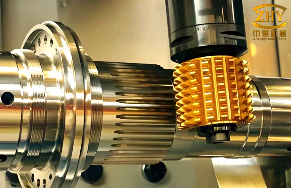
I begin from the machining principle. In the generating method, the cutter head is mounted on a cutter spindle, and the workpiece is mounted on a workpiece spindle. The cradle and cutter spindle have an eccentric arrangement. Their combined motion creates a virtual generating gear. The workpiece rotates in mesh with this virtual generating gear. The cutter edges cut one tooth slot after another. During this process, the gear machining state is influenced by many factors, including spindle speed, feed rate, cutter wear, structural stiffness, thermal deformation, and assembly clearance. These factors are not independent. They interact and produce complex vibration behavior. I analyze this behavior as a nonlinear and non-stationary process.
I model the cutting contact as a spring-mass-damper system. The cutter edge displacement is affected by the cutting force, the contact stiffness, and the damping. I write the general vibration equation as
$$ M \ddot{x} + C \dot{x} + K(t)x = K_r(t)E + K(t)E(t) $$
where \(M\) is the equivalent mass, \(C\) is the damping, \(K(t)\) is the time-varying stiffness, \(x\) is the cutter edge displacement, \(K_r(t)\) is the cutting stiffness, and \(E(t)\) represents the excitation caused by the cutting process. In gear machining, multiple cutter edges enter and leave the workpiece. The number of engaged edges changes with the cutter head rotation. The meshing impact and the variation of cutting force generate broadband vibration. When the machine state changes from normal to chatter, the vibration amplitude, energy distribution, and frequency composition change significantly. I use these changes to identify the machine state.
I classify the vibration sources of the spiral bevel gear milling machine into two groups. The first group is internal and unavoidable. It includes the periodic excitation from the cutter spindle, the workpiece spindle, the cradle motion, and the gear meshing impact. The second group is external and partly avoidable. It includes foundation vibration, nearby machine tools, coolant flow, and environmental noise. For reliability assessment, I am mainly interested in the internal vibration because it reflects the machine condition during gear machining.
| Vibration source | Origin | Effect on gear machining | Observability |
|---|---|---|---|
| Cutter spindle rotation | Motor, bearing, spindle assembly | Periodic cutting force variation | High |
| Workpiece spindle rotation | Servo drive, gear train, bearing | Indexing error and tooth surface waviness | High |
| Cradle motion | Guideway, worm gear, servo system | Generating motion error | Medium |
| Cutting impact | Intermittent edge engagement | High-frequency impact and chatter | High |
| Structural deformation | Thermal and force-induced deformation | Tooth profile deviation | Low to medium |
The signal acquisition system I built contains three parts: sensors, a data acquisition card, and a data acquisition platform. I use piezoelectric accelerometers because they are suitable for contact measurement on a rotating spindle housing. The sensitivity is \(100\,\mathrm{mV/g}\), and the measurement range is \(\pm 50\,g\). I use a three-axis accelerometer to obtain vibration in the X, Y, and Z directions. I mount the sensor close to the cutter spindle because this location is close to the cutting zone and has sufficient stiffness. I use a compact reconfigurable input-output controller and a dynamic signal acquisition module. I develop the acquisition software with a virtual instrument environment. The sampling frequency is \(10240\,\mathrm{Hz}\). Each acquisition contains \(102400\) points. I divide the signal into \(20\) segments, and each segment contains \(2048\) points. I collect \(20\) segments for the normal state and \(20\) segments for the chatter state. In this way, I obtain \(40\) vibration signal samples for state analysis.
| Parameter | Value | Purpose |
|---|---|---|
| Sensor sensitivity | \(100\,\mathrm{mV/g}\) | Convert vibration acceleration to voltage |
| Measurement range | \(\pm 50\,g\) | Cover normal and chatter amplitudes |
| Sampling frequency | \(10240\,\mathrm{Hz}\) | Capture high-frequency impact components |
| Segment length | \(2048\) points | Provide stable feature samples |
| Segments per state | \(20\) | Support statistical comparison |
| Measurement directions | X, Y, Z | Capture spatial vibration behavior |
Before feature extraction, I reduce noise in the raw vibration signal. Because the signal from gear machining is nonlinear and non-stationary, simple frequency filtering may remove useful components. I use singular value decomposition for denoising. I construct a Hankel matrix from the one-dimensional signal. For a signal \(x_1, x_2, \ldots, x_N\), the Hankel matrix is
$$ H = \begin{bmatrix}
x_1 & x_2 & \cdots & x_n \\
x_2 & x_3 & \cdots & x_{n+1} \\
\vdots & \vdots & \ddots & \vdots \\
x_m & x_{m+1} & \cdots & x_N
\end{bmatrix} $$
where \(N = m + n – 1\). I choose the row number \(m\) and column number \(n\) to make the matrix approximately square. I use
$$ m = \begin{cases}
N/2, & N \text{ even}, \\
(N+1)/2, & N \text{ odd}.
\end{cases} $$
Then I decompose the Hankel matrix as
$$ H = U S V^T $$
where \(U\) and \(V\) are orthogonal matrices and \(S\) is a non-negative diagonal matrix. The large singular values are mainly related to the useful signal, and the small singular values are mainly related to noise. I apply a singular value difference spectrum to separate them. I set the small singular values to zero and reconstruct the matrix. Finally, I convert the reconstructed matrix back to a one-dimensional signal. This denoised signal retains the main vibration characteristics while suppressing background noise.
After denoising, I extract features in both the time domain and the time-frequency domain. Time-domain analysis is simple and intuitive. It reflects amplitude, energy, impact, and waveform shape. I use both dimensional and dimensionless indicators. The dimensional indicators include mean, root mean square, variance, root amplitude, absolute mean, maximum, minimum, peak, and peak-to-peak value. The dimensionless indicators include skewness, kurtosis, waveform factor, peak factor, impulse factor, clearance factor, and kurtosis factor. These indicators describe different aspects of the vibration signal during gear machining.
| Dimensional indicator | Expression | Physical meaning |
|---|---|---|
| Mean | \(\bar{x} = \frac{1}{N}\sum_{i=1}^{N}x_i\) | Static component |
| Root mean square | \(x_{\mathrm{rms}} = \left(\frac{1}{N}\sum_{i=1}^{N}x_i^2\right)^{1/2}\) | Vibration intensity |
| Variance | \(\sigma^2 = \frac{1}{N}\sum_{i=1}^{N}(x_i-\bar{x})^2\) | Dispersion degree |
| Root amplitude | \(x_r = \left(\frac{1}{N}\sum_{i=1}^{N}|x_i|^{1/2}\right)^2\) | Low-amplitude energy |
| Absolute mean | \(x_{\mathrm{abs}} = \frac{1}{N}\sum_{i=1}^{N}|x_i|\) | Average absolute level |
| Peak-to-peak | \(x_{p-p} = \max(x_i)-\min(x_i)\) | Maximum excursion |
| Dimensionless indicator | Expression | Physical meaning |
|---|---|---|
| Skewness | \(S = \frac{\frac{1}{N}\sum_{i=1}^{N}x_i^3}{\left(\frac{1}{N}\sum_{i=1}^{N}x_i^2\right)^{3/2}}\) | Asymmetry of amplitude distribution |
| Kurtosis | \(K = \frac{\frac{1}{N}\sum_{i=1}^{N}x_i^4}{\left(\frac{1}{N}\sum_{i=1}^{N}x_i^2\right)^2}\) | Impulsiveness of the signal |
| Waveform factor | \(K_w = \frac{x_{\mathrm{rms}}}{x_{\mathrm{abs}}}\) | Waveform shape |
| Peak factor | \(C = \frac{\max|x_i|}{x_{\mathrm{rms}}}\) | Peak intensity |
| Impulse factor | \(I = \frac{\max|x_i|}{x_{\mathrm{abs}}}\) | Impact content |
| Clearance factor | \(L = \frac{\max|x_i|}{x_r}\) | Clearance-related impact |
Although time-domain indicators are useful, they cannot fully describe the time-frequency distribution of a non-stationary vibration signal from gear machining. Therefore, I apply local mean decomposition. This method decomposes a complex signal into a set of product functions and a residual. Each product function contains a frequency component and an envelope component. The decomposition reduces the influence of endpoint effects and is suitable for nonlinear signals. The main steps are as follows.
For the original signal \(x(t)\), I find all local extrema. I calculate the local mean \(m_{11}(t)\) and the local envelope estimate \(a_{11}(t)\) from adjacent extrema. I subtract the local mean from the original signal:
$$ h_{11}(t) = x(t) – m_{11}(t) $$
I demodulate \(h_{11}(t)\) by the envelope estimate:
$$ s_{11}(t) = \frac{h_{11}(t)}{a_{11}(t)} $$
If \(a_{12}(t) \ne 1\), I repeat the process with \(s_{11}(t)\) as the new signal. The iteration stops when the envelope estimate approaches one. The envelope signal is the product of all envelope estimates:
$$ a_1(t) = a_{11}(t)a_{12}(t)\cdots a_{1n}(t) $$
The first product function is
$$ PF_1(t) = a_1(t)s_{1n}(t) $$
I subtract \(PF_1(t)\) from \(x(t)\) and continue the decomposition until the residual becomes monotonic. The final expression is
$$ x(t) = \sum_{d=1}^{k} PF_d(t) + u_k(t) $$
where \(PF_d(t)\) is the \(d\)-th product function and \(u_k(t)\) is the final residual. I calculate the energy of each product function as
$$ E_{PF_d} = \sum_{i=1}^{M} PF_d^2(i) $$
where \(M\) is the number of sampling points in the product function. The energy values reflect the distribution of vibration energy in different frequency bands. For the normal state, the X direction decomposes into four main product functions, the Y direction into five, and the Z direction into four. For the chatter state, the X direction decomposes into five, the Y direction into five, and the Z direction into five. To keep the feature dimension consistent, I select the energy values of the first four product functions as time-frequency features.
| State and direction | Number of product functions | Selected features |
|---|---|---|
| Normal X | 4 | PF1 to PF4 energy |
| Normal Y | 5 | PF1 to PF4 energy |
| Normal Z | 4 | PF1 to PF4 energy |
| Chatter X | 5 | PF1 to PF4 energy |
| Chatter Y | 5 | PF1 to PF4 energy |
| Chatter Z | 5 | PF1 to PF4 energy |
After I extract many features, I need to select the features that are most sensitive to the machine state. A feature with weak sensitivity increases computation and reduces the discriminative ability of the feature set. I use distance evaluation technology to quantify feature sensitivity. For a feature \(p\), I calculate the average within-class distance as
$$ d_{t,p} = \frac{1}{M_t(M_t-1)}\sum_{l,m=1, l \ne m}^{M_t}|q_{m,t,p}-q_{l,t,p}| $$
where \(t\) is the state class, \(M_t\) is the number of samples in class \(t\), and \(q_{m,t,p}\) is the feature value of sample \(m\). The average within-class distance over all states is
$$ d_p^w = \frac{1}{T}\sum_{t=1}^{T}d_{t,p} $$
The within-class variation factor is
$$ v_p^w = \frac{\max(d_{t,p})}{\min(d_{t,p})} $$
The average feature value for class \(t\) is
$$ u_{t,p} = \frac{1}{M_t}\sum_{m=1}^{M_t}q_{m,t,p} $$
The between-class distance is
$$ d_p^b = \frac{1}{T(T-1)}\sum_{s,t=1, s \ne t}^{T}|u_{t,p}-u_{s,p}| $$
The between-class variation factor is
$$ v_p^b = \frac{\max|u_{t,p}-u_{s,p}|}{\min|u_{t,p}-u_{s,p}|} $$
I define the compensation factor as
$$ \lambda_p = \left(\frac{\max(v_p^w)}{\max(v_p^b)} + \frac{\max(v_p^b)}{\max(v_p^w)}\right)^{-1} $$
Finally, the distance evaluation index is
$$ \alpha_p = \lambda_p \frac{d_p^b}{d_p^w} $$
A larger \(\alpha_p\) means that the feature is more sensitive to the machine state. I calculate the distance evaluation indices for the extracted features. The results are shown in the following table.
| Feature | Distance evaluation index | Feature | Distance evaluation index |
|---|---|---|---|
| Mean | 0.3238 | Peak factor | 1.3827 |
| Root mean square | 7.3438 | Impulse factor | 1.6394 |
| Root amplitude | 5.8173 | Clearance factor | 2.0894 |
| Absolute mean | 6.4619 | Kurtosis factor | 3.1746 |
| Skewness | 4.3822 | PF1 energy | 5.8332 |
| Kurtosis | 5.8311 | PF2 energy | 13.4263 |
| Variance | 6.2317 | PF3 energy | 1.0821 |
| Peak-to-peak | 4.8693 | PF4 energy | 0.4589 |
| Waveform factor | 0.1289 | — | — |
From this table, I select the root mean square and the PF2 energy as the state-sensitive feature indicators. The root mean square reflects the vibration intensity, and the PF2 energy reflects the energy concentration in a sensitive frequency band. Both indicators show clear separation between the normal state and the chatter state during gear machining. I use these two indicators as response covariates in the reliability model.
For reliability modeling, I use a proportional hazards model. This model relates the state covariates to the hazard rate. It does not require failure data from a large population and can use condition monitoring data. The general form is
$$ h(t;Z) = h_0(t)\exp(\gamma^T Z) $$
where \(h_0(t)\) is the baseline hazard function, \(Z\) is the covariate vector, and \(\gamma\) is the regression parameter vector. I assume that the baseline hazard follows a Weibull distribution because the Weibull distribution is flexible and widely used for mechanical reliability. The baseline hazard and reliability functions are
$$ h_0(t) = \frac{\beta}{\eta}\left(\frac{t}{\eta}\right)^{\beta-1} $$
$$ R_0(t) = \exp\left[-\left(\frac{t}{\eta}\right)^\beta\right] $$
where \(\beta\) is the shape parameter and \(\eta\) is the scale parameter. When the two selected covariates \(Z_1\) and \(Z_2\) are included, the Weibull proportional hazards model becomes
$$ h(t;Z) = \frac{\beta}{\eta}\left(\frac{t}{\eta}\right)^{\beta-1}\exp(\gamma_1 Z_1 + \gamma_2 Z_2) $$
The cumulative hazard is
$$ H(t;Z) = \int_0^t h(u;Z)du = \left(\frac{t}{\eta}\right)^\beta \exp(\gamma_1 Z_1 + \gamma_2 Z_2) $$
The reliability function is
$$ R(t;Z) = \exp[-H(t;Z)] = \exp\left[-\left(\frac{t}{\eta}\right)^\beta \exp(\gamma_1 Z_1 + \gamma_2 Z_2)\right] $$
This expression provides the reliability of the machine at time \(t\) under the current vibration state. The covariates are derived from the vibration signal during gear machining. Therefore, the reliability changes when the machine state changes. This is the main advantage of the proportional hazards model for condition-based reliability assessment.
I estimate the unknown parameters by the maximum likelihood method. For a data set with \(n\) observations and \(r\) failures, the likelihood function is
$$ L(\beta,\eta,\gamma) = \prod_{i=1}^{r} f(t_i;Z_i)\prod_{i=1}^{n} R(t_i;Z_i) $$
For the Weibull proportional hazards model, the log-likelihood function is
$$ \ell(\beta,\eta,\gamma) = \sum_{i=1}^{r}\left[\ln\left(\frac{\beta}{\eta}\right) + (\beta-1)\ln\left(\frac{t_i}{\eta}\right) + \gamma^T Z_i\right] – \sum_{i=1}^{n}\left(\frac{t_i}{\eta}\right)^\beta \exp(\gamma^T Z_i) $$
I take partial derivatives with respect to \(\beta\), \(\eta\), \(\gamma_1\), and \(\gamma_2\), set them to zero, and solve the resulting equations. Because the equations are nonlinear, I use an iterative optimization algorithm. The estimated parameters are shown in the following table.
| Parameter | Meaning | Estimated value |
|---|---|---|
| \(\beta\) | Weibull shape parameter | 13.58 |
| \(\eta\) | Weibull scale parameter | 121.66 |
| \(\gamma_1\) | Regression coefficient for root mean square | 7.62 |
| \(\gamma_2\) | Regression coefficient for PF2 energy | 8.34 |
Using these parameters, I calculate the reliability for each sample. The reliability values for the normal state and the chatter state form two distinct layers. The normal state has higher reliability, and the chatter state has lower reliability. This result shows that the vibration-based proportional hazards model can distinguish machine states during gear machining. The model also provides a quantitative reliability index instead of a qualitative state label. When the reliability drops below a maintenance threshold, I can plan maintenance before a severe failure occurs.
I also evaluate the machine from the perspective of product quality. The gear measuring center provides the normal deviation of the tooth surface. I process the measured data to obtain the machining error distribution along the tooth width and around the gear circumference. The error distribution reflects the combined effect of machine vibration, cutter wear, thermal deformation, and indexing error. When the machine is in a normal state, the error distribution is relatively stable. When the machine is in a chatter state, the error distribution fluctuates more strongly. Therefore, the gear quality data can be used as an indirect indicator of machine reliability during gear machining.
I construct a behavior sequence for each machining error distribution. For a single tooth surface, the measured error values form a sequence
$$ X = (x(1), x(2), \ldots, x(n)) $$
I use grey relational analysis to compare the similarity between sequences. The absolute relational degree is calculated from the difference between a reference sequence and a comparison sequence. The grey relational coefficient is
$$ \xi_{0i}(k) = \frac{\min_i\min_k |x_0(k)-x_i(k)| + \rho \max_i\max_k |x_0(k)-x_i(k)|}{|x_0(k)-x_i(k)| + \rho \max_i\max_k |x_0(k)-x_i(k)|} $$
where \(x_0\) is the reference sequence, \(x_i\) is the comparison sequence, and \(\rho\) is the resolution coefficient. The grey relational degree is
$$ r_{0i} = \frac{1}{n}\sum_{k=1}^{n}\xi_{0i}(k) $$
A larger relational degree means that the two error distribution curves are more similar. I use this value to evaluate three aspects of process reliability: retention, repeatability, and consistency. Retention compares the error distribution of one tooth surface with an ideal equal-value sequence. Repeatability compares the same tooth surface from different gear workpieces. Consistency compares the concave and convex surfaces of the same tooth.
| Evaluation type | Comparison sequence | Reference object |
|---|---|---|
| Retention | Minimum absolute error sequence | Same tooth and same surface of one gear |
| Repeatability | Sequence with highest retention | Same tooth and same surface of different gears |
| Consistency | Sequence with highest retention | Different surfaces of the same tooth |
For retention, I compare the actual error distribution with the equal-value sequence formed by the minimum absolute error. The results for two gear workpieces under different machine states are shown below.
| Tooth number | Gear A concave retention | Gear A convex retention | Gear B concave retention | Gear B convex retention |
|---|---|---|---|---|
| 1 | 0.756 | 0.834 | 0.729 | 0.882 |
| 2 | 0.732 | 0.822 | 0.886 | 0.796 |
| 3 | 0.742 | 0.862 | 0.816 | 0.864 |
| 4 | 0.781 | 0.841 | 0.823 | 0.841 |
The retention values are relatively high for both gear workpieces. This indicates that the machine maintains the error distribution along the tooth surface to a certain degree. However, the retention value alone is not enough to determine the machine reliability. I also evaluate repeatability. I compare the same tooth surface from two gear workpieces machined under different machine states. The results are shown below.
| Tooth number | Concave repeatability | Convex repeatability |
|---|---|---|
| 1 | 0.318 | 0.418 |
| 2 | 0.329 | 0.831 |
| 3 | 0.248 | 0.768 |
| 4 | 0.278 | 0.516 |
The repeatability values are lower than the retention values. The concave surfaces show especially low repeatability. This means that the same tooth surface produced under different machine states is not highly similar. The convex surfaces have higher repeatability than the concave surfaces, but the values still vary. This result suggests that the inner cutter and outer cutter produce different error behavior during gear machining. The machine needs maintenance to improve the repeatability of the process.
I then evaluate consistency by comparing the concave and convex surfaces of the same tooth. The results are shown below.
| Tooth number | Gear A consistency | Gear B consistency |
|---|---|---|
| 1 | 0.732 | 0.213 |
| 2 | 0.681 | 0.247 |
| 3 | 0.529 | 0.285 |
| 4 | 0.746 | 0.236 |
Gear A has higher consistency than Gear B. Gear A was machined when the machine was in the normal state, while Gear B was machined when the machine was in the chatter state. The lower consistency of Gear B indicates that the concave and convex surfaces deviate from each other more strongly when the machine is unstable. This is consistent with the vibration-based reliability result. When the machine reliability decreases, the gear machining quality becomes less consistent.
By combining the vibration-based reliability model and the quality-based grey relational evaluation, I obtain a more complete reliability assessment. The vibration features provide a real-time state indicator. The Weibull proportional hazards model converts this indicator into a reliability value. The gear error data provide a product-level verification. The grey relational analysis shows whether the process is stable in terms of retention, repeatability, and consistency. In my view, this combination is useful for heavy machine tools because failure data are often scarce, but condition data and quality data are available during gear machining.
| Assessment level | Data source | Method | Output |
|---|---|---|---|
| Signal level | Vibration acceleration | SVD and LMD | State-sensitive features |
| Feature level | Time and time-frequency features | Distance evaluation | RMS and PF2 energy |
| Reliability level | Selected features | Weibull proportional hazards | State-based reliability |
| Quality level | Tooth surface error | Grey relational analysis | Retention, repeatability, consistency |
The main equations used in my reliability assessment can be summarized as follows. The selected feature vector is
$$ Z = [Z_1, Z_2]^T = [x_{\mathrm{rms}}, E_{PF2}]^T $$
The Weibull proportional hazards reliability function is
$$ R(t;Z) = \exp\left[-\left(\frac{t}{\eta}\right)^\beta \exp(\gamma_1 Z_1 + \gamma_2 Z_2)\right] $$
With the estimated parameters, the model becomes
$$ R(t;Z) = \exp\left[-\left(\frac{t}{121.66}\right)^{13.58} \exp(7.62 Z_1 + 8.34 Z_2)\right] $$
This equation allows me to compute the reliability of the machine at a given time when the root mean square and PF2 energy are known. A higher feature value indicates a more severe vibration state, which reduces the reliability. A lower feature value indicates a more stable state, which increases the reliability. In gear machining, the operator can monitor these features and estimate the current reliability without waiting for a failure to occur.
I also note several limitations in my study. First, I collected data from a limited number of machine states. The normal state and the chatter state are two representative conditions, but they do not cover the entire life cycle. A full life-cycle test from commissioning to overhaul would provide more information. Second, I used vibration signals as the main condition data. In actual gear machining, current, temperature, acoustic emission, and cutting force also contain useful information. Multi-sensor fusion could improve the reliability assessment. Third, my experiments were performed under controlled conditions. In a production environment, the working conditions are more variable, and the signal-to-noise ratio may be lower. The robustness of the method should be further tested. Fourth, I evaluated vibration reliability and quality reliability separately. Building a direct mapping between the two would help verify their consistency and provide a unified reliability index.
Despite these limitations, the results support the following conclusions. The vibration signal from gear machining contains rich state information. Singular value decomposition can suppress noise while preserving the main waveform. Local mean decomposition can extract time-frequency energy features from nonlinear and non-stationary signals. Distance evaluation can identify the most sensitive features. The root mean square and PF2 energy are effective indicators for distinguishing normal and chatter states. The Weibull proportional hazards model can convert these indicators into a reliability function. The estimated parameters show that both covariates have a strong effect on the hazard rate. The reliability curves for the normal and chatter states are clearly separated.
The gear error data provide another view of machine reliability. The grey relational analysis of retention, repeatability, and consistency shows that the machine produces better quality when it is in a stable state. When chatter occurs, the error distribution becomes less repeatable and less consistent. This agrees with the vibration-based reliability result. Therefore, I can use both condition monitoring and product quality to support maintenance decisions in gear machining.
| Conclusion number | Finding | Practical meaning |
|---|---|---|
| 1 | SVD reduces noise in non-stationary vibration signals | Improves feature reliability |
| 2 | LMD energy features reflect state changes | Captures time-frequency behavior |
| 3 | Distance evaluation selects RMS and PF2 energy | Reduces feature dimension |
| 4 | Weibull proportional hazards model gives state-based reliability | Supports condition-based maintenance |
| 5 | Grey relational analysis quantifies quality stability | Verifies process reliability from product data |
For future work, I plan to extend the experiment over a longer period and collect data from more machine states. I will also add current and temperature sensors to the acquisition platform. I intend to study feature fusion methods that combine vibration, current, and temperature data. In addition, I will investigate how to map the vibration-based reliability index to the quality-based reliability index. Such a mapping would allow a single reliability value to represent both machine condition and product quality during gear machining. I believe this direction is valuable for heavy machine tools, especially for spiral bevel gear milling machines, because their motion coupling and cutting mechanism make reliability assessment difficult but also make condition monitoring highly informative.
In summary, I have developed a reliability assessment framework for a spiral bevel gear milling machine based on vibration characteristics and machining quality. The framework includes signal acquisition, SVD denoising, time-domain and time-frequency feature extraction, distance-based feature selection, Weibull proportional hazards modeling, maximum likelihood parameter estimation, and grey relational quality evaluation. The results show that the machine state during gear machining can be quantified by vibration features and that the resulting reliability value is consistent with the quality of the machined gear. This approach provides a practical way to monitor machine reliability in real time and to support maintenance planning for gear machining equipment.