
In my work on aviation spiral bevel gears, I focused on the gear cutting stage that follows near-net forging and precedes heat treatment. I treated the large wheel of an aviation spiral bevel gear as the main object because its tooth geometry, contact behavior, and manufacturing accuracy strongly influence noise, load capacity, and service life. The overall process route I considered is near-net forging, gear cutting, heat treatment, precision grinding, and surface strengthening. This article concentrates on the gear cutting operation and on how cutting parameters affect tooth-surface deformation and residual stress.
I used a first-person research approach: I built the geometric model, I constructed the finite element models, I ran single-factor and Box-Behnken simulations, I fitted response surface models, I optimized the cutting parameters, and I validated the predictions through gear cutting experiments. The central variables in my study are cutting speed, feed per revolution, and cutting depth. The central responses are tooth-surface deformation and residual stress along the depth direction.
Geometric and Kinematic Basis of Gear Cutting
For the large wheel, I applied the standard geometric relationships of spiral bevel gears. The pitch diameters, cone angles, face cone, root cone, and cutter generating surface provide the basis for both the three-dimensional model and the gear cutting simulation. I calculated the main geometric parameters with the equations below.
$$d_1 = m z_1, \qquad d_2 = m z_2$$
$$\tan\delta_2 = \frac{z_2 \sin\Sigma}{z_1 + z_2 \cos\Sigma}, \qquad \delta_1 = \Sigma – \delta_2$$
$$\delta_{i1} = \delta_1 – \gamma_1 – \Delta\gamma, \qquad \delta_{i2} = \delta_2 – \gamma_2 – \Delta\gamma$$
$$\delta_{a1} = 90^\circ – \delta_2, \qquad \delta_{a2} = 90^\circ – \delta_1$$
$$R_e = \frac{d_2}{2\sin\delta_2}$$
$$h_{a1} = (h_a^* + \xi)m, \qquad h_{a2} = (h_a^* – \xi)m$$
$$h_{f1} = (h_f^* + c – \xi)m, \qquad h_{f2} = (h_a^* + c – \xi)m$$
$$\tan\gamma_1 = \frac{h_{f1}}{R_e}, \qquad \tan\gamma_2 = \frac{h_{f2}}{R_e}$$
$$D_1 = d_1 + 2h_{a1}\cos\delta_1, \qquad D_2 = d_2 + 2h_{a2}\cos\delta_2$$
The geometric parameters I used for the large wheel are summarized in Table 1. These values define the blank, the tooth surface, and the machine settings required for gear cutting.
| Parameter | Value | Parameter | Value |
|---|---|---|---|
| Module, mm | 3 | Number of teeth | 44 |
| Hand of spiral | Left | Face width, mm | 20.2 |
| Addendum coefficient | 0.85 | Pressure angle, deg | 20 |
| Mean spiral angle, deg | 35 | Shaft angle, deg | 90 |
| Pitch diameter, mm | 132 | Outer cone distance, mm | 69.73 |
| Face cone angle, deg | 73.39 | Mounting distance, mm | 27 |
For the forming method used in gear cutting of the large wheel, the cutter rotates about the cutter-head axis while the blank remains fixed during one tooth slot. The cutting edge generates a conical surface. I expressed the cutter generating surface as follows.
$$r_t(\mu,\theta)=
\begin{bmatrix}
r_c \pm \mu \sin\alpha_m \cos\theta\\
r_c \pm \mu \sin\alpha_m \sin\theta\\
-\mu \cos\alpha_m
\end{bmatrix}$$
Here, \(\mu\) and \(\theta\) are parameters of a moving point on the cutting edge, \(r_c\) is the cutter tip radius, \(\alpha_m\) is the profile angle, and the upper and lower signs correspond to the inner and outer cutters. I also expressed the face cone of the large wheel as
$$r_a(p,\beta)=
\begin{bmatrix}
p\cos\delta_a\\
p\sin\delta_a\sin\beta\\
p\sin\delta_a\cos\beta
\end{bmatrix}$$
where \(p\) and \(\beta\) are parameters on the face cone, and \(\delta_a\) is the face cone angle. To connect the cutter surface to the workpiece, I used coordinate transformations between the cutter system, the machine system, and the gear system.
$$r_m = M_{mt} r_t$$
$$r_{am} = M_{mf} M_{f2} M_{2a} r_a$$
The intersection of the face cone and the cutter generating surface gives the contact line during gear cutting:
$$L = r_{am}(p,\beta,z_j) – r_m(\mu,\theta)=0$$
The radial cutter position and angular cutter position are
$$S = \sqrt{H^2+V^2}, \qquad q = \arctan\left(\frac{V}{H}\right)$$
The entry and exit angles of the cutter are approximated by
$$\theta_{st} \approx \arcsin\left(\frac{B}{2r_0\cos\beta_m}\right) – \frac{\pi}{2} + k\beta_m$$
$$\theta_{ex} \approx \arcsin\left(\frac{B}{2r_0\cos\beta_m}\right) + \frac{\pi}{2} + k\beta_m$$
For the instantaneous uncut chip geometry in gear cutting, I calculated the chip thickness and width for the outer cutter, inner cutter, and top edge. The main cutting edge values are
$$h_{ew}=2f_z\sin\alpha_e, \qquad b_{ew}=u_{ej}(\theta_j,z_j)$$
$$h_{iw}=2f_z\sin\alpha_i, \qquad b_{iw}=u_{ij}(\theta_j,z_j)$$
and the top-edge values are
$$h_w=2f_z, \qquad b_w=S_b$$
where \(f_z\) is the feed per tooth, \(S_b\) is the top width of the cutter, and \(u_{ej}\) and \(u_{ij}\) are derived from the intersection equation. These quantities guided my selection of gear cutting parameters for the finite element simulations.
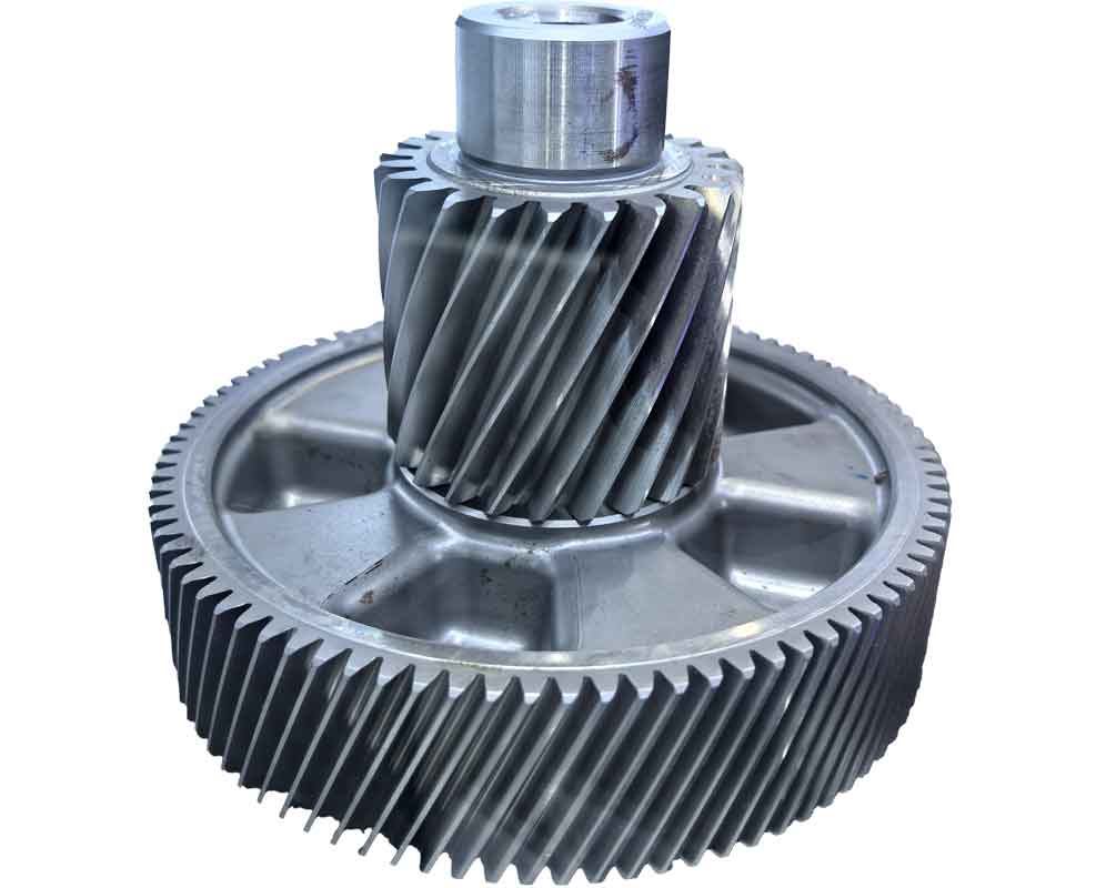
The gear cutting arrangement I modeled is shown below. The relative motion between the cutter head and the large wheel defines the forming method, and the cutting edges remove the tooth slot in a cyclic manner.
Finite Element Material Models for Gear Cutting
I used AISI 4340 steel for the gear because it combines high strength, toughness, and hardenability. Its physical properties are listed in Table 2. These properties were used in the forging simulation, the gear cutting deformation simulation, and the oblique gear cutting residual stress simulation.
| Property | Value | Property | Value |
|---|---|---|---|
| Density, T/mm\(^3\) | \(7.83\times10^{-9}\) | Yield limit, MPa | 792 |
| Elastic modulus, MPa | \(2\times10^5\) | Ultimate strength, MPa | 980 |
| Poisson ratio | 0.29 | Thermal conductivity, W/m/°C | 38 |
| Specific heat, kJ/T/°C | \(4.77\times10^8\) | Expansion coefficient, mm/°C | \(3.2\times10^{-5}\) |
| Melting point, °C | 1519.85 | Reference temperature, °C | 25 |
For the thermo-mechanical behavior during gear cutting, I applied the Johnson-Cook constitutive model:
$$\sigma=\left[A+B(\varepsilon^{pl})^n\right]\left[1+C\ln\left(\frac{\dot{\varepsilon}^{pl}}{\dot{\varepsilon}_0}\right)\right](1-\hat{\theta}^m)$$
where \(\sigma\) is equivalent stress, \(\varepsilon^{pl}\) is equivalent plastic strain, \(\dot{\varepsilon}^{pl}\) is plastic strain rate, \(\dot{\varepsilon}_0\) is reference strain rate, and \(\hat{\theta}\) is the homologous temperature. The homologous temperature is defined as
$$\hat{\theta}=
\begin{cases}
0, & TT_m
\end{cases}$$
The Johnson-Cook parameters I used for AISI 4340 are given in Table 3.
| \(A\), MPa | \(B\), MPa | \(n\) | \(C\) | \(m\) |
|---|---|---|---|---|
| 792 | 510 | 0.26 | 0.014 | 1.03 |
For chip formation and material separation in gear cutting, I used the Johnson-Cook damage criterion. The damage parameter is
$$\omega=\sum\left(\frac{\Delta\bar{\varepsilon}^{pl}}{\bar{\varepsilon}_f^{pl}}\right)$$
and failure occurs when \(\omega>1\). The failure strain is
$$\bar{\varepsilon}_f^{pl}=[D_1+D_2\exp(-D_3\eta)]\left[1+D_4\ln\left(\frac{\dot{\bar{\varepsilon}}}{\dot{\varepsilon}_0}\right)\right][1+D_5\hat{\theta}]$$
where \(\eta=-p/q\) is stress triaxiality. The failure parameters are listed in Table 4.
| \(D_1\) | \(D_2\) | \(D_3\) | \(D_4\) | \(D_5\) |
|---|---|---|---|---|
| 0.05 | 3.44 | 2.12 | 0.002 | 0.61 |
I also used a fracture-energy-based damage evolution to reduce mesh dependence during gear cutting:
$$G_f=\int_{\varepsilon_0^{pl}}^{\varepsilon_f^{pl}}\sigma_y\,d\varepsilon^{pl}L=\int_0^{u_f^{pl}}\sigma_y\,du^{pl}$$
Forging Model for Initial Stress State Before Gear Cutting
Because the large wheel is produced by near-net forging before gear cutting, I built a forging model to extract the initial residual stress state. I created the forging blank, upper die, and lower die in a three-dimensional CAD environment. To reduce computation time, I used a 1/12 sector with symmetry boundary conditions. I treated the blank as an elastic-plastic body at 900 °C, the dies as rigid bodies at 200 °C, the friction coefficient as 0.25, the forging speed as 20 mm/s, and the air convection coefficient as 0.02 N/s/mm/°C. After forging and cooling, I extracted the residual stress on the tooth surface near the pitch circle and mapped it into the gear cutting model as an initial stress field. The extraction path and initial stress trend were used as preprocessing data for the subsequent gear cutting residual stress analysis.
Tooth-Surface Deformation Model for Gear Cutting
For tooth-surface deformation, I built a single-tooth-slot gear cutting model. The cutter was treated as a rigid body, and the tooth blank was treated as an elastic-plastic body with AISI 4340 properties. I used tetrahedral elements for the workpiece, opened heat transfer and heat generation, set the friction coefficient to 0.2, fixed the gear bottom, and defined the cutter motion according to the selected gear cutting parameters. After each simulation, I extracted the total displacement on the tooth surface. I selected five tooth lines from root to tip along the tooth height, and nine lines along the face width, producing 45 data points. The maximum value among these points was taken as the tooth-surface deformation for that simulation.
I then conducted single-factor simulations. The levels are shown in Table 5.
| Factor | Level 1 | Level 2 | Level 3 | Level 4 |
|---|---|---|---|---|
| Cutting speed \(v\), m/min | 80 | 100 | 120 | 140 |
| Cutting depth \(a\), mm | 1.0 | 1.5 | 2.0 | 2.5 |
| Feed \(f\), mm/r | 0.2 | 0.3 | 0.4 | 0.5 |
The single-factor results showed clear trends. As feed increased, tooth-surface deformation increased. As cutting depth increased, deformation also increased, but the change was smaller. As cutting speed increased, deformation first increased and then decreased. I attributed this behavior to the competition between mechanical loading, friction-induced heat, and thermal softening in the gear cutting zone. Higher feed and depth remove more material and increase the mechanical load, while higher speed increases friction and heat but also promotes thermal softening and faster chip evacuation.
To quantify the combined effects, I used a Box-Behnken design. The simulation matrix and deformation results are shown in Table 6.
| Run | \(v\), m/min | \(a\), mm | \(f\), mm/r | Deformation \(\delta\), μm |
|---|---|---|---|---|
| 1 | 140 | 1.00 | 0.35 | 20.181 |
| 2 | 110 | 2.50 | 0.50 | 31.370 |
| 3 | 110 | 2.50 | 0.20 | 21.600 |
| 4 | 80 | 1.75 | 0.50 | 29.001 |
| 5 | 110 | 1.75 | 0.35 | 22.600 |
| 6 | 80 | 1.00 | 0.35 | 19.595 |
| 7 | 140 | 2.50 | 0.35 | 18.500 |
| 8 | 80 | 1.75 | 0.20 | 19.050 |
| 9 | 80 | 2.50 | 0.35 | 22.819 |
| 10 | 110 | 1.75 | 0.35 | 22.401 |
| 11 | 110 | 1.00 | 0.20 | 20.229 |
| 12 | 110 | 1.00 | 0.50 | 29.900 |
| 13 | 140 | 1.75 | 0.50 | 27.065 |
| 14 | 110 | 1.75 | 0.35 | 22.500 |
| 15 | 140 | 1.75 | 0.20 | 17.201 |
I fitted a quadratic response surface model for tooth-surface deformation:
$$\hat{\delta}=\beta_0+\sum_{i=1}^{3}\beta_i x_i+\sum_{i=1}^{3}\sum_{j=1}^{3}\beta_{ij}x_i x_j+\sum_{i=1}^{3}\beta_{ii}x_i^2+\varepsilon_c$$
The fitted deformation model was
$$\hat{\delta}=12.58-0.6673v+5.190a+61.72f-0.002734v^2-0.417a^2-135.11f^2-0.05450va-0.0048vf+0.220af$$
The analysis of variance for the deformation model is given in Table 7. The model was highly significant, and the adjusted coefficient of determination was close to the ordinary coefficient of determination, which indicated good fit.
| Source | DF | Sum of squares | Mean square | F value | P value |
|---|---|---|---|---|---|
| Model | 9 | 269.352 | 29.9279 | 602.84 | 0.0001 |
| Error | 5 | 0.248 | 0.0496 | ||
| Total | 14 | 269.600 | |||
| \(R^2\) | 98.91% | ||||
| \(R^2_{adj}\) | 96.74% |
Using the response optimizer, I minimized the tooth-surface deformation under the constraints
$$\min(\delta)
\begin{cases}
80 \leq v \leq 140\\
1.0 \leq a \leq 2.5\\
0.2 \leq f \leq 0.5
\end{cases}$$
The optimal gear cutting conditions for minimum deformation were \(a=2.5\) mm, \(f=0.2303\) mm/r, and \(v=140\) m/min. The predicted minimum deformation was \(16.6734\) μm.
Residual Stress Model for Gear Cutting
For residual stress, the length scale is much smaller than the whole tooth. A full three-dimensional gear cutting model with a fine mesh over the entire gear would be computationally expensive and difficult for stress extraction near the surface. Therefore, I used an equivalent three-dimensional oblique gear cutting model. I selected a micro-element on the tooth surface that experiences the same local cutting conditions as the actual forming method. I set the rake angle to \(15^\circ\), the clearance angle to \(6^\circ\), the edge inclination angle to \(5^\circ\), and the tool tip radius to \(0.02\) mm. I assigned AISI 4340 to the workpiece and carbide to the tool, used a friction coefficient of \(0.2\), and applied a coupled thermo-mechanical analysis.
In the oblique gear cutting model, the cutting force components are
$$F_t=K_{tc}da_p t_c+K_{te}da_p$$
$$F_f=K_{fc}da_p t_c+K_{fe}da_p$$
$$F_r=K_{rc}da_p t_c+K_{re}da_p$$
where \(da_p\) is the axial width of the oblique cutting element, \(t_c\) is the uncut chip thickness, \(K_{tc}\), \(K_{fc}\), and \(K_{rc}\) are shearing force coefficients, and \(K_{te}\), \(K_{fe}\), and \(K_{re}\) are ploughing force coefficients. The shearing force coefficients can be expressed as
$$K_{tc}=\frac{\tau_s(\cos\theta_n+\tan\theta_i\tan\beta)}{\cos\theta_n\cos\phi_n[\cos^2(\phi_n+\theta_n)+\tan^2\theta_i\sin^2\phi_n]}$$
$$K_{fc}=\frac{\tau_s\sin\theta_n}{\cos\theta_n\cos\phi_n[\cos^2(\phi_n+\theta_n)+\tan^2\theta_i\sin^2\phi_n]}$$
$$K_{rc}=\frac{\tau_s(\tan\theta_i-\cos\theta_n\tan\beta)}{\cos\theta_n\cos\phi_n[\cos^2(\phi_n+\theta_n)+\tan^2\theta_i\sin^2\phi_n]}$$
The shear flow stress is derived from the Johnson-Cook model:
$$\tau_s=\frac{1}{\sqrt{3}}\left[A+B\left(\frac{\varepsilon}{\sqrt{3}}\right)^n\right]\left[1+C\ln\left(\frac{\dot{\varepsilon}}{\dot{\varepsilon}_0}\right)\right]\left[1-\left(\frac{T-T_0}{T_m-T_0}\right)^m\right]$$
I extracted residual stress along the depth direction at a plane 2.7 mm from the left end face of the workpiece. On each path, I sampled stress values every 0.02 mm in the depth direction and averaged three paths. The stress component \(S_{11}\) was used as the residual stress in the cutting direction.
I first examined the influence of the initial forging residual stress. The comparison showed that the two stress curves had the same general shape. The surface was tensile, and the stress quickly became compressive with increasing depth. However, when the initial forging stress was applied, the maximum tensile stress was smaller and the maximum compressive stress was larger. Deeper inside the workpiece, the case without initial stress tended toward zero, while the case with initial stress remained compressive. This confirmed that the initial stress state produced by near-net forging should not be ignored in gear cutting residual stress analysis.
I then studied cutting speed, feed, and cutting depth by single-factor simulations. The results are summarized in Table 8.
| Parameter | Effect on surface tensile stress | Effect on subsurface compressive stress | Effect on stress layer depth |
|---|---|---|---|
| Cutting speed \(v\) | Increases as \(v\) increases | Decreases as \(v\) increases | Slight change |
| Feed \(f\) | Increases as \(f\) increases | Increases as \(f\) increases | Increases as \(f\) increases |
| Cutting depth \(a\) | Slight increase | Small change | Small change |
The thermal-mechanical coupling mechanism explains these trends. Near the machined surface, the heat generated by plastic deformation and friction dominates, producing tensile stress after cooling. Deeper below the surface, mechanical loading dominates and produces compressive stress. The final residual stress profile is the superposition of thermal stress, mechanical stress, and the initial stress state. In my simulations, the surface was tensile, then rapidly became compressive, reached a compressive peak, and finally approached a stable value deeper inside the material.
I used a Box-Behnken design for residual stress as well. The simulation matrix and stress results are shown in Table 9, where \(S_1\) is the maximum residual tensile stress and \(S_2\) is the maximum residual compressive stress.
| Run | \(v\), m/min | \(a\), mm | \(f\), mm/r | \(S_1\), MPa | \(S_2\), MPa |
|---|---|---|---|---|---|
| 1 | 140 | 1.00 | 0.35 | 287.261 | -310.382 |
| 2 | 110 | 2.50 | 0.50 | 327.251 | -343.221 |
| 3 | 110 | 2.50 | 0.20 | 227.031 | -260.907 |
| 4 | 80 | 1.75 | 0.50 | 311.205 | -363.342 |
| 5 | 110 | 1.75 | 0.35 | 282.635 | -321.862 |
| 6 | 80 | 1.00 | 0.35 | 265.625 | -342.498 |
| 7 | 140 | 2.50 | 0.35 | 303.991 | -284.649 |
| 8 | 80 | 1.75 | 0.20 | 207.373 | -318.221 |
| 9 | 80 | 2.50 | 0.35 | 270.516 | -347.691 |
| 10 | 110 | 1.75 | 0.35 | 282.635 | -321.862 |
| 11 | 110 | 1.00 | 0.20 | 221.101 | -291.957 |
| 12 | 110 | 1.00 | 0.50 | 311.657 | -353.952 |
| 13 | 140 | 1.75 | 0.50 | 339.498 | -345.521 |
| 14 | 110 | 1.75 | 0.35 | 282.635 | -321.862 |
| 15 | 140 | 1.75 | 0.20 | 257.602 | -242.541 |
I fitted quadratic response surface models for \(S_1\) and \(S_2\):
$$\hat{S}_1=\beta_0+\sum_{i=1}^{3}\beta_i x_i+\sum_{i=1}^{3}\sum_{j=1}^{3}\beta_{ij}x_i x_j+\sum_{i=1}^{3}\beta_{ii}x_i^2+\varepsilon_c$$
$$\hat{S}_2=\beta_0+\sum_{i=1}^{3}\beta_i x_i+\sum_{i=1}^{3}\sum_{j=1}^{3}\beta_{ij}x_i x_j+\sum_{i=1}^{3}\beta_{ii}x_i^2+\varepsilon_c$$
The fitted models were
$$\hat{S}_1=74.2+0.026v+9.9a+624.9f+0.00345v^2-7.06a^2-306.8f^2-0.1315va-1.219vf+21.0af$$
$$\hat{S}_2=-450.8+1.944v+1.6a+210.0f-0.00281v^2-6.07a^2-123f^2-0.3436va-3.270vf-39.4af$$
The analysis of variance for the tensile stress model is given in Table 10, and that for the compressive stress model is given in Table 11.
| Source | DF | Sum of squares | Mean square | F value | P value |
|---|---|---|---|---|---|
| Model | 9 | 20641.5 | 2293.5 | 159.95 | 0.0001 |
| Error | 5 | 71.7 | 23.9 | ||
| Total | 14 | 22713.2 | |||
| \(R^2\) | 99.03% | ||||
| \(R^2_{adj}\) | 94.46% |
| Source | DF | Sum of squares | Mean square | F value | P value |
|---|---|---|---|---|---|
| Model | 9 | 22376.1 | 2486.2 | 132.55 | 0.0001 |
| Error | 5 | 93.8 | 18.8 | ||
| Total | 14 | 22469.9 | |||
| \(R^2\) | 98.83% | ||||
| \(R^2_{adj}\) | 93.32% |
For residual stress, tensile stress is generally detrimental, while compressive stress is beneficial. Therefore, I optimized the gear cutting parameters to minimize the maximum tensile stress and maximize the maximum compressive stress:
$$\min(S_1), \qquad \max(S_2)$$
$$\begin{cases}
80 \leq v \leq 140\\
1.0 \leq a \leq 2.5\\
0.2 \leq f \leq 0.5
\end{cases}$$
The optimal gear cutting parameters for residual stress were \(a=2.5\) mm, \(f=0.2037\) mm/r, and \(v=80\) m/min. The predicted minimum tensile stress was \(207.4106\) MPa, and the predicted maximum compressive stress was \(322.2280\) MPa. The main effect analysis showed that feed had the greatest influence on residual stress, followed by cutting speed, while cutting depth had the smallest influence. This ranking is important for practical gear cutting because it indicates that feed control is the most effective way to regulate the final stress state.
Experimental Validation of Gear Cutting Predictions
I validated the finite element models and response surface predictions through a set of gear cutting experiments on a CNC machine. I mounted the forged large-wheel blank on the indexing table, clamped it, installed the cutter head, adjusted the relative position, and ran the NC program containing spindle speed, feed, and cutting depth. After gear cutting, I measured tooth-surface deviation on a gear measuring machine. I selected five tooth slots to reduce measurement uncertainty. For residual stress, I cut the gear into single teeth by wire electrical discharge machining, keeping the cutting path far from the measured tooth surface to minimize stress release. I then measured residual stress by X-ray diffraction and removed thin surface layers by electrolytic polishing to obtain the depth profile.
The measured and predicted deformation values are compared in Table 12. The maximum relative error was 8.39%, and the errors were below 10% for all measured slots. The experimental values were generally larger than the predicted values, which I attributed to machine vibration, clamping variation, and minor tool wear during actual gear cutting.
| Slot | Measured deformation, μm | Predicted deformation, μm | Relative error, % |
|---|---|---|---|
| 1 | 17.7000 | 16.6734 | 5.80 |
| 2 | 18.2000 | 16.6734 | 8.39 |
| 3 | 17.3000 | 16.6734 | 3.62 |
| 4 | 15.8000 | 16.6734 | 5.53 |
| 5 | 17.4000 | 16.6734 | 4.18 |
The residual stress comparison is given in Table 13. The measured depth profiles followed the same trend as the simulations: tensile at the surface, rapid transition to compressive stress, a compressive peak, and gradual stabilization. The maximum relative error for the tensile and compressive peaks was 6.17%, which confirmed that the oblique gear cutting model and the response surface predictions were reliable.
| Group | Measured \(S_1\), MPa | Predicted \(S_1\), MPa | Error, % | Measured \(S_2\), MPa | Predicted \(S_2\), MPa | Error, % |
|---|---|---|---|---|---|---|
| 1 | 204.302 | 207.411 | 1.52 | 326.620 | 322.228 | 1.34 |
| 2 | 199.942 | 207.411 | 4.26 | 311.351 | 322.228 | 3.83 |
| 3 | 195.355 | 207.411 | 6.17 | 303.535 | 322.228 | 6.16 |
| 4 | 196.473 | 207.411 | 5.57 | 308.326 | 322.228 | 4.51 |
Discussion
My results show that gear cutting parameters do not affect deformation and residual stress in exactly the same way. For deformation, feed and cutting speed are the dominant factors, while cutting depth has a smaller effect. For residual stress, feed is the most influential parameter, followed by cutting speed, and cutting depth is again the least influential. This difference occurs because deformation is controlled mainly by the global mechanical load and the amount of material removed, whereas residual stress is controlled by the local thermal-mechanical history and by the depth of the plastically deformed layer.
The depth profile of residual stress is a direct consequence of the coupled thermal and mechanical fields during gear cutting. The surface experiences high temperature and severe plastic strain, which tends to produce tensile stress after cooling. Below the surface, the mechanical pressure and plastic deformation are still significant, but the thermal effect is weaker, so compressive stress dominates. The transition depth and the peak compressive stress depend on feed, speed, tool geometry, and the initial forging stress. In my simulations, applying the forging-induced initial stress shifted the entire profile, reducing the tensile peak and increasing the compressive peak. This means that process-chain integration is essential for accurate prediction of gear cutting residual stress.
The optimized parameters for minimum deformation and for the most favorable residual stress are not identical. Minimum deformation was obtained at high cutting speed, high cutting depth, and moderate feed. The most favorable residual stress was obtained at low cutting speed, high cutting depth, and low feed. In practical gear cutting of aviation spiral bevel gears, the final choice should therefore be based on the dominant requirement. If dimensional accuracy is the primary concern, the deformation-minimizing combination is preferred. If fatigue life and surface integrity are the primary concerns, the residual-stress-optimizing combination is preferred. A compromise can also be reached by weighting the two responses according to the service conditions.
Conclusions
I established a complete modeling and validation framework for gear cutting of near-net-formed aviation spiral bevel gears before heat treatment. The main conclusions are as follows.
First, the tooth-surface deformation in gear cutting increases with feed and cutting depth. As cutting speed increases, deformation first increases and then decreases. Feed and cutting speed have a stronger influence than cutting depth. The fitted response surface model for deformation is significant, and the optimal parameters for minimum deformation are \(a=2.5\) mm, \(f=0.2303\) mm/r, and \(v=140\) m/min, giving a predicted minimum deformation of \(16.6734\) μm.
Second, the residual stress profile after gear cutting is tensile at the machined surface, rapidly becomes compressive with depth, reaches a compressive peak, and finally approaches a stable value. The maximum tensile stress increases with cutting speed, feed, and cutting depth. The maximum compressive stress increases with feed, decreases with cutting speed, and changes non-monotonically with cutting depth. Feed has the greatest effect on residual stress, followed by cutting speed, while cutting depth has the smallest effect.
Third, the initial residual stress from near-net forging must be included in the gear cutting model. When it is included, the tensile peak decreases, the compressive peak increases, and the deeper region remains compressive. This improves the agreement between simulation and experiment.
Fourth, the response surface models for both deformation and residual stress are reliable. The optimal gear cutting parameters for minimizing tensile stress and maximizing compressive stress are \(a=2.5\) mm, \(f=0.2037\) mm/r, and \(v=80\) m/min, giving \(S_1=207.4106\) MPa and \(S_2=322.2280\) MPa.
Fifth, the experimental validation supports the models. The maximum relative error for deformation was 8.39%, and the maximum relative error for the residual stress peaks was 6.17%. The measured residual stress profiles followed the simulated profiles in both magnitude and trend. I therefore conclude that the finite element models, the oblique gear cutting simplification, and the response surface prediction models are accurate enough to support parameter selection for gear cutting of aviation spiral bevel gears.
Overall, this work provides a practical basis for controlling deformation and residual stress during gear cutting after near-net forming and before heat treatment. It also shows that gear cutting parameter optimization should consider both dimensional accuracy and surface integrity, because the two objectives can require different cutting conditions. The framework I developed can be extended to other gear sizes, tool geometries, and initial stress states, and it can be integrated into a full process-chain control strategy for high-performance spiral bevel gears.