
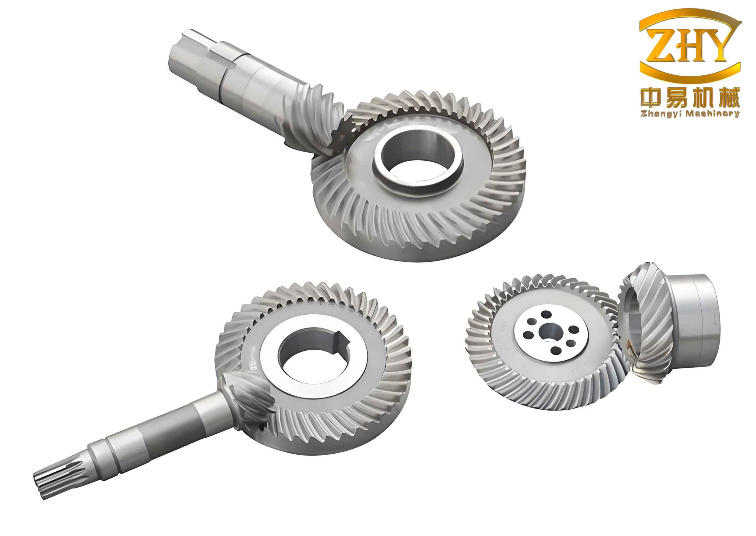
In the realm of power transmission, especially for automotive applications requiring high torque capacity and smooth operation in a compact package, the hyperboloid gear, or hypoid gear, stands out. Compared to spiral bevel gears, hyperboloid gears offer superior strength and quieter performance due to their offset axes, which allow for larger pinion diameters and more gradual tooth engagement. As engineering demands push for higher precision, lower noise, and greater load-bearing capabilities, advanced manufacturing methods become paramount. Among Gleason’s established techniques, the HGT (Hypoid Generator Tilt) method is particularly significant. While HFT (formate) methods are valued for efficiency, HGT employs a generating process for the gear, offering a higher degree of control and adjustment potential during cutting, ultimately leading to gears of exceptional quality. This article provides a comprehensive, first-person exploration of the HGT hyperboloid gear, from its precise mathematical modeling and three-dimensional simulation to loaded tooth contact analysis and experimental validation.
1. Mathematical Modeling of Tooth Surfaces
The foundation for analyzing any hyperboloid gear lies in an accurate mathematical description of its tooth surfaces. We derive these surfaces based on the kinematic principles of the traditional cradle-type hypoid generator, which provides an intuitive and geometrically clear model.
1.1 Coordinate Systems and Kinematics
The generation process involves the relative motion between the cutter head (simulating the imaginary generating gear) and the workpiece. A series of coordinate systems are established to describe this motion, which are then condensed into fundamental transformation matrices. The machine setup parameters, such as cutter radius, machine root angle, sliding base setting, and work offset, are embedded within these transformations.
The primary coordinate systems include:
- Cutter Coordinate System (Sc): Fixed to the rotating cutter head.
- Machine Cradle Coordinate System (Sm): Fixed to the cradle, which rotates with a generating roll angle \(\phi_c\).
- Workpiece Coordinate System (Sw): Fixed to the gear or pinion being cut, rotating with its own work rotation angle \(\phi_w\).
The relationship between the cradle roll and work rotation is defined by the generating ratio, forming the core of the generating motion. The general transformation from a point on the cutter to a point on the workpiece is given by:
$$ \mathbf{r}_w(\theta, \phi_c, \phi_w) = \mathbf{M}_{wc}(\theta, \phi_c, \phi_w) \cdot \mathbf{r}_c(\theta) $$
$$ \mathbf{n}_w(\theta, \phi_c, \phi_w) = \mathbf{L}_{wc}(\theta, \phi_c, \phi_w) \cdot \mathbf{n}_c(\theta) $$
where \(\mathbf{r}_w\) and \(\mathbf{n}_w\) are the position vector and unit normal vector of the workpiece surface point, \(\mathbf{r}_c\) and \(\mathbf{n}_c\) are those of the cutter surface point, \(\theta\) is the cutter blade profile parameter, and \(\mathbf{M}_{wc}\) and \(\mathbf{L}_{wc}\) are the composite transformation and rotation matrices encompassing all machine settings.
1.2 Working Surface Equation Derivation
The working tooth surfaces of the hyperboloid gear pair are generated by the straight-sided blades of the cutter head. The surface of the cutter blade is a conical surface. In the cutter coordinate system \(S_c\), the family of these blade surfaces can be represented as:
$$ \mathbf{r}_c(s, \theta) = \begin{bmatrix} (r_c \pm s \sin \alpha) \cos \theta \\ (r_c \pm s \sin \alpha) \sin \theta \\ \mp s \cos \alpha \\ 1 \end{bmatrix} $$
where \(r_c\) is the cutter point radius, \(s\) is the distance along the blade, \(\alpha\) is the cutter blade pressure angle, and \(\theta\) is the rotational parameter of the cutter head. The signs (\(\pm, \mp\)) correspond to the convex and concave sides of the gear and pinion, selected appropriately for inner (concave) and outer (convex) blades.
Applying the coordinate transformation \(\mathbf{M}_{wc}\) yields the family of surfaces on the workpiece:
$$ \mathbf{r}_w(s, \theta, \phi_c, \phi_w) = \mathbf{M}_{wc}(\phi_c, \phi_w) \cdot \mathbf{r}_c(s, \theta) $$
This represents all points that the cutter sweeps relative to the workpiece. The actual generated tooth surface is the envelope of this family of surfaces. According to the theory of gearing, the envelope condition, or the equation of meshing, is given by the scalar product of the relative velocity vector and the surface normal being zero:
$$ f(s, \theta, \phi_c, \phi_w) = \mathbf{n}_w \cdot \mathbf{v}_w^{(cw)} = 0 $$
Here, \(\mathbf{n}_w\) is the unit normal to the workpiece surface family and \(\mathbf{v}_w^{(cw)}\) is the relative velocity of the cutter with respect to the workpiece in the workpiece coordinate system. The relative velocity is derived from the kinematics of the machine:
$$ \mathbf{v}_w^{(cw)} = \frac{d\mathbf{r}_w}{dt} = \left( \frac{\partial \mathbf{M}_{wc}}{\partial \phi_c} \dot{\phi}_c + \frac{\partial \mathbf{M}_{wc}}{\partial \phi_w} \dot{\phi}_w \right) \mathbf{r}_c $$
Given the generating relationship \(\phi_w = R_{atio} \cdot \phi_c\), the equation of meshing can be expressed as a function of the parameters \(s, \theta, \phi_c\).
$$ f(s, \theta, \phi_c) = 0 $$
The system of equations defining the hyperboloid gear tooth surface is therefore:
$$ \begin{cases}
\mathbf{r}_w = \mathbf{r}_w(s, \theta, \phi_c) \\
f(s, \theta, \phi_c) = 0
\end{cases} $$
By eliminating one parameter (typically \(\phi_c\)), we obtain the explicit representation of the tooth surface \(\mathbf{r}_w(s, \theta)\). This process is performed separately for the gear and pinion, and for their convex and concave flanks, using the corresponding machine settings and cutter parameters.
1.3 Fillet (Root Transition) Surface Equation Derivation
The root fillet of the hyperboloid gear is generated by the tip rounding (or tip corner) of the cutter blade. Accurate modeling of this fillet is crucial for finite element stress analysis. The tip rounding is typically a circular arc. In a local coordinate system \(S_t\) attached to the blade tip, the arc is defined as:
$$ \mathbf{r}_t(\lambda) = \begin{bmatrix} \pm r_t \cos \lambda \\ 0 \\ r_t \sin \lambda \\ 1 \end{bmatrix} $$
where \(r_t\) is the tip radius and \(\lambda\) is the parameter along the arc (e.g., \(-\pi/2 \le \lambda \le 0\)). This arc is first positioned on the cutter head. Its location depends on the blade’s basic geometry: the point width, the blade pressure angle \(\alpha\), and the tip radius \(r_t\). The position of the arc center point \(P_c\) in the cutter coordinate system \(S_c\) is:
$$ \mathbf{P}_c^c = \begin{bmatrix} r_c \pm r_t (1 – \sin \alpha) \tan \alpha \\ 0 \\ \mp r_t \cos \alpha \\ 1 \end{bmatrix} $$
The transformation from the tip arc coordinate system \(S_t\) to the cutter system \(S_c\) involves a translation to \(P_c^c\) and potentially a rotation. The resulting cutter fillet surface family is:
$$ \mathbf{r}_c^{fillet}(\lambda, \theta) = \mathbf{M}_{ct}(\theta) \cdot \mathbf{r}_t(\lambda) $$
Following the same envelope procedure as for the working surface—transforming to the workpiece system and applying the equation of meshing—yields the mathematical model for the root fillet surface of the hyperboloid gear.
$$ \begin{cases}
\mathbf{r}_w^{fillet} = \mathbf{M}_{wc}(\phi_c) \cdot \mathbf{M}_{ct}(\theta) \cdot \mathbf{r}_t(\lambda) \\
f^{fillet}(\lambda, \theta, \phi_c) = \mathbf{n}_w^{fillet} \cdot \mathbf{v}_w^{(cw)} = 0
\end{cases} $$
The complete tooth model is the union of the working surface and its adjoining fillet surface.
| Parameter Category | Symbol | Description | Typical Role |
|---|---|---|---|
| Basic Gear Data | \(z_1, z_2\) | Number of pinion & gear teeth | Defines gear ratio |
| \(\Sigma\) | Shaft angle | Typically 90° | |
| \(E\) | Offset distance | Key feature of hyperboloid gear | |
| \(\beta_m\) | Mean spiral angle | Affects smoothness and axial thrust | |
| Cutter Parameters | \(r_{c}\) | Cutter point radius | Controls tooth lengthwise curvature |
| \(\alpha_o, \alpha_i\) | Outer/Inner blade pressure angle | Determines side contact pressure | |
| \(r_{t}\) | Tip rounding radius | Defines root fillet geometry | |
| \(\theta_{tip}\) | Tip angle parameter | Defines the extent of the fillet arc | |
| Blade Profile | Straight-sided / Skived | Defines the basic generating surface | |
| Machine Settings (HGT) | \(R_{atio}\) | Generating ratio (Roll) | Links cradle and work rotation |
| \(\gamma_m\) | Machine root angle | Orients workpiece relative to cradle | |
| \(X_B, X_D\) | Sliding Base & Blank Offset | Positions workpiece radially/axially | |
| \(i, j\) | Tilt & Swivel Angles | Unique to HGT/HGM; adjust contact path | |
| \(S_{R}\) | Cradle Radial Setting | Radial distance of cutter from cradle center | |
| \(q\) | Helical Motion Ratio | For modified roll |
2. Development of the 3D Geometric Simulation Model
With the mathematical models for both the working and fillet surfaces of the hyperboloid gear pair in hand, the next step is to construct a precise three-dimensional digital model. This model serves as the essential foundation for all subsequent computer-aided engineering (CAE) analyses.
The process begins by implementing the derived surface equations into a computational algorithm. For a given surface (e.g., gear concave flank), the code solves for a dense set of coordinate points \(\mathbf{r}_w(u, v)\), where \(u\) and \(v\) are independent surface parameters (e.g., \(s\) and a solved-for \(\theta\)). The algorithm must handle the different parameter ranges for the active profile and the root fillet, ensuring a continuous transition. This point cloud data is then exported in a standard format (e.g., IGES, STEP, or a simple XYZ list).
This data is imported into commercial 3D CAD or specialized gear software. Using advanced surface fitting techniques—such as Non-Uniform Rational B-Splines (NURBS)—the discrete points are interpolated to create smooth, accurate, and water-tight surface patches. These patches are then stitched together to form a solid model of a single tooth. Through pattern replication about the gear axis, the complete gear and pinion solids are generated. Finally, these components are virtually assembled according to their specified shaft angle and offset, creating the final 3D simulation model of the hyperboloid gear drive. This digital twin is critical for visualization, interference checking, and most importantly, as the input for tooth contact and stress analysis.
3. Tooth Contact Analysis (TCA) and Loaded Tooth Contact Analysis (LTCA)
The performance of a hyperboloid gear set is predominantly evaluated through contact analysis. We first examine the unloaded condition and then proceed to the more realistic loaded scenario.
3.1 Unloaded Tooth Contact Analysis (TCA)
TCA simulates the meshing of the theoretically perfect gear pair under zero torque. The goal is to predict the contact pattern (or bearing contact) and the unloaded transmission error (TE). The fundamental equation of TCA states that at the point of contact between two meshing tooth surfaces \(\mathbf{r}_1(u_1, \theta_1)\) and \(\mathbf{r}_2(u_2, \theta_2)\), their position vectors and unit normals must coincide in a fixed coordinate system \(S_f\).
$$ \begin{cases}
\mathbf{r}_f^{(1)}(u_1, \theta_1, \phi_1) = \mathbf{r}_f^{(2)}(u_2, \theta_2, \phi_2) \\
\mathbf{n}_f^{(1)}(u_1, \theta_1, \phi_1) = \mathbf{n}_f^{(2)}(u_2, \theta_2, \phi_2)
\end{cases} $$
Here, \(\phi_1\) and \(\phi_2\) are the rotation angles of the pinion and gear, related by the ratio \(\phi_2 = (z_1/z_2) \phi_1\). This system yields five independent scalar equations (since \(|\mathbf{n}|=1\) reduces one condition) for six unknowns \((u_1, \theta_1, \phi_1, u_2, \theta_2, \phi_2)\). By choosing one parameter, say the pinion rotation \(\phi_1\), as the input, the system can be solved iteratively (e.g., using the Newton-Raphson method) for the remaining five, identifying the contact point path across the tooth surface.
The transmission error \(\Delta \phi_2\) is the deviation from perfect kinematic motion:
$$ \Delta \phi_2(\phi_1) = \phi_2(\phi_1) – \frac{z_1}{z_2} \phi_1 $$
A well-designed hyperboloid gear aims for a low-amplitude, parabolic-shaped TE curve, which minimizes vibration excitation. The instantaneous contact ellipse is calculated at each point based on the principal curvatures and relative curvature of the two surfaces at that point. The TCA results provide the initial, unloaded contact pattern on the tooth flank, which is a primary indicator of the quality of the manufacturing setup.
3.2 Loaded Tooth Contact Analysis (LTCA)
LTCA is a critical simulation that predicts the behavior of the hyperboloid gear pair under actual operating loads. It accounts for tooth bending, shear, and contact deformations, which significantly alter the contact pattern and transmission error compared to the unloaded state. The analysis assumes a series of discrete potential contact points along the predicted path of contact. The fundamental equations governing LTCA are the compatibility of deformations and the equilibrium of forces.
Let \(p_i\) be the normal load at the \(i\)-th potential contact point, \(w_i\) be the initial geometric separation (including unloaded transmission error) at that point, \(\delta_{ij}\) be the combined bending and contact compliance influence coefficient (deflection at point \(i\) due to a unit load at point \(j\)), \(\theta\) be the relative angular approach of the gears due to deformation, and \(r_i\) be the moment arm. The system can be formulated as follows:
- Deformation Compatibility: The final gap \(d_i\) at each point after loading must be zero if contact occurs (\(p_i > 0\)), or positive if contact is lost (\(p_i = 0\)).
$$ \sum_{j=1}^{n} \delta_{ij} p_j + w_i = \theta r_i + d_i, \quad i=1,…,n $$ - Force and Moment Equilibrium:
$$ \sum_{i=1}^{n} p_i = F_{total}, \quad \sum_{i=1}^{n} p_i r_i = T $$
where \(F_{total}\) is the total normal force and \(T\) is the applied torque. - Contact Conditions (Complementarity):
$$ p_i \ge 0, \quad d_i \ge 0, \quad p_i \cdot d_i = 0 $$
This forms a Linear Complementarity Problem (LCP) or can be solved as a constrained optimization problem (e.g., minimizing strain energy). The compliance matrix \(\mathbf{\Delta} = [\delta_{ij}]\) is often pre-calculated using a detailed finite element model of a single tooth pair for various load positions.
Solving this system for increasing input torque yields the loaded contact pattern (usually larger and shifted towards the toe and heel compared to the unloaded pattern), the load distribution among simultaneous contact lines, and the loaded transmission error. A key observation in the analysis of HGT hyperboloid gears is their tendency to develop edge contact under high torque. This occurs when the contact ellipse, enlarged by deformation, extends beyond the tooth boundaries at the toe, heel, top, or root. Edge contact is highly undesirable as it leads to elevated stress concentrations, increased noise, and potential premature failure.
| Performance Metric | Unloaded TCA (Theoretical) | Loaded LTCA (Simulated Real Condition) | Significance |
|---|---|---|---|
| Contact Pattern | Centered, narrow, elliptical shape. Location is sensitive to machine settings. | Larger, often shifted towards toe/heel. Shape may distort. Edge contact may appear under high load. | LTCA shows the actual operating contact area, crucial for assessing durability and risk of localized wear. |
| Transmission Error (TE) | Low-amplitude, often parabolic curve. Defines inherent kinematic excitation. | Amplitude is reduced and waveform is flattened under optimal load. Can increase if edge contact occurs. | Loaded TE is the true source of vibratory excitation. A smooth, low TE is critical for quiet operation. |
| Load Sharing | Not applicable (single pair contact assumed in kinematics). | Shows distribution among 2 or 3 tooth pairs. Calculates load sharing ratio and maximum single-tooth load. | Determines the actual safety factor and root stress. High contact ratio leads to better load sharing. |
| Sensitivity | Sensitive to geometric errors (misalignment). | Sensitive to both geometric errors and system stiffness (shafts, bearings, housing). | LTCA provides a complete system-level performance prediction, essential for robust design. |
4. Manufacturing Verification and Experimental Insights
The ultimate validation of the mathematical models and simulations for the HGT hyperboloid gear comes from physical manufacturing and testing. A gear pair is cut on a hypoid generator (or a modern CNC machine emulating its kinematics) using the calculated HGT machine settings. The cutting process is monitored to ensure parameters like tilt (\(i\)) and swivel (\(j\)) are correctly implemented.
After cutting, the gears are typically subjected to a rolling test on a gear testing machine, such as a Gleason No. 504 or similar tester. A light marking compound is applied to the tooth flanks. As the gears roll under very light load, they imprint a contact pattern. This experimental pattern is then compared with the LTCA-predicted pattern. Key aspects of the comparison include:
- Pattern Location and Size: The experimental pattern should correlate well with the LTCA prediction for a corresponding low-torque condition.
- Pattern Shape: It should be a well-formed oval, avoiding bi-concave (hourglass) shapes or excessive diagonal orientation.
- Absence of Edge Contact at Nominal Load: Under the designated test load, the pattern should remain within the tooth boundaries.
Our analysis and verification for a typical HGT hyperboloid gear pair (90° shaft angle, 38mm offset) revealed two major conclusions that align with general observations for such gears. First, the hyperboloid gear design inherently promotes a high contact ratio. The LTCA results confirmed multiple tooth-pair contact throughout the mesh cycle, leading to smooth power transmission and low vibration levels. Second, the analysis clearly identified a load threshold for edge contact. While the contact pattern remained well-contained at lower torques, the simulation predicted that when the gear torque exceeded a specific value (e.g., 500 N·m in our case), the contact ellipse would deform and extend beyond the tooth edge at the exit region. This phenomenon was also observed as a tendency in the physical rolling test under higher loads, confirming the predictive power of the LTCA model. Understanding this threshold is vital for defining the operational limits of the gear set and for initiating redesign if the threshold is too low for the application.
5. Conclusion
This comprehensive guide has detailed the complete process for the design, simulation, and analysis of hyperboloid gears manufactured via the HGT method. Beginning with the derivation of precise mathematical models for both working and fillet surfaces based on cradle-type generator kinematics, we established the foundation for creating an accurate 3D digital twin of the gear pair. This model enables advanced computational analyses. We then detailed the two-stage performance evaluation process: Tooth Contact Analysis (TCA) for predicting unloaded kinematics and contact paths, and Loaded Tooth Contact Analysis (LTCA) for simulating real-world operating conditions, including deformations, load distribution, and the critical phenomenon of edge contact.
The successful correlation between LTCA predictions and physical cutting tests validates the entire modeling chain. The key outcomes for HGT hyperboloid gears—high contact ratio for smoothness and a defined load limit for edge contact—highlight both their performance advantages and a primary design constraint. The methodologies presented here, from the fundamental equation of meshing $$f(s, \theta, \phi_c)=0$$ to the loaded contact compliance equations, provide a reliable and essential framework. This framework is the crucial prerequisite for any subsequent in-depth study of hyperboloid gear performance, including finite element analysis for root and contact stress, dynamic system modeling for noise and vibration prediction, and advanced optimization of machine settings for tailored performance. Mastery of these principles is fundamental to advancing the design and application of these complex yet highly efficient power transmission components.