
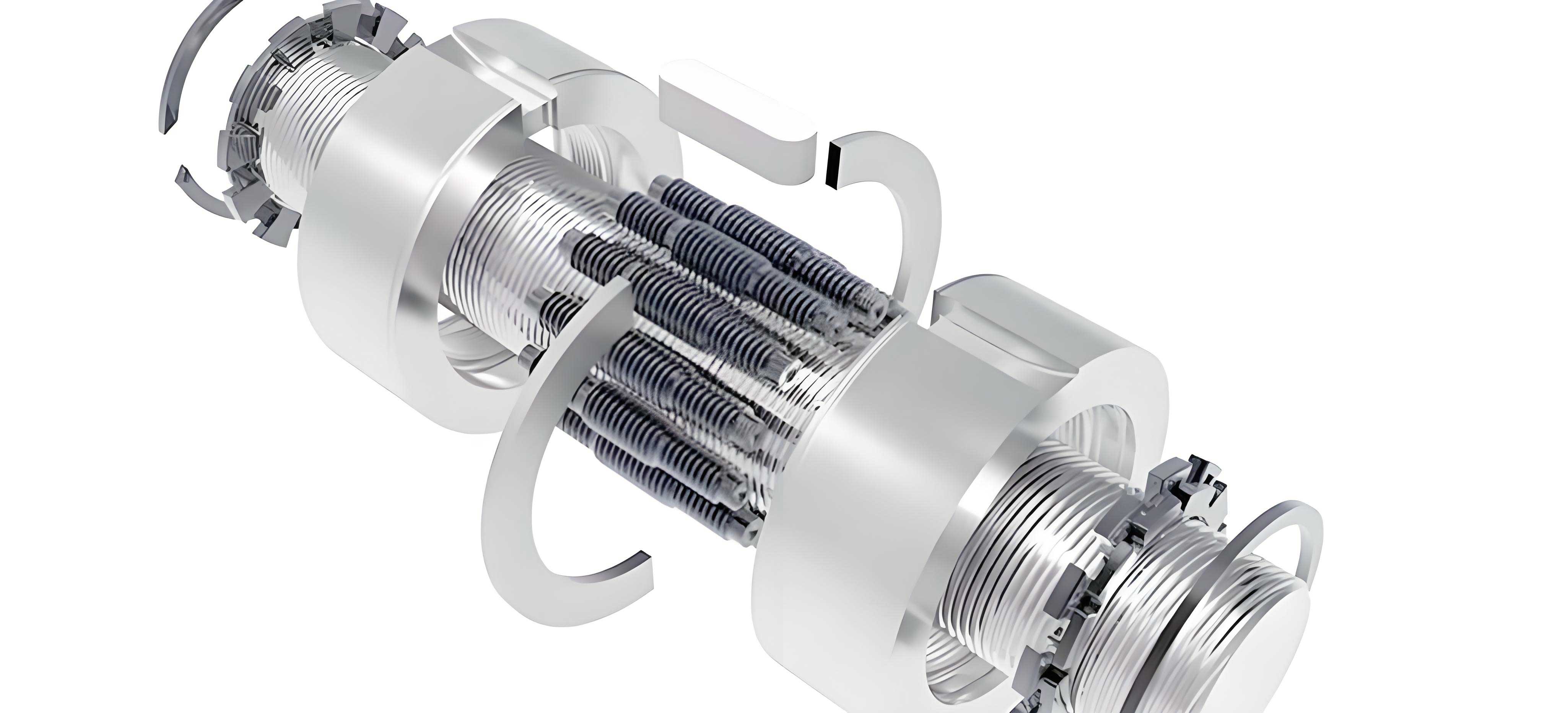
The planetary roller screw assembly is a critical mechanism for converting rotational motion into linear motion, renowned for its superior load capacity, precision, and longevity. Its performance hinges on the complex elastic contact interactions between the threaded surfaces of its primary components: the central screw, the planetary rollers, and the surrounding nut. Accurate modeling of these contact zones, particularly their shape and stress distribution, is fundamental for design optimization and reliability prediction.
This article delves into a detailed contact mechanics analysis of the standard-type planetary roller screw assembly. We move beyond simplified methods to incorporate a crucial geometric parameter often overlooked: the angle between the principal planes of the contacting bodies at their point of contact. By rigorously applying differential geometry and Hertzian contact theory, we establish a comprehensive framework for evaluating contact characteristics, revealing the influence of structural parameters with greater precision.
Geometric Modeling and Principal Curvature Calculation
The foundation of our contact analysis lies in the precise mathematical description of the helical raceway surfaces. Individual coordinate systems are established for the screw, roller, and nut, with the z-axis coinciding with each component’s axis of rotation. The position of any point on a thread surface can be represented in its part-specific coordinates as \( (r_{pi}, \theta_{pi}, z_{pi}) \), where the subscript \( i = s, r, n \) denotes the screw, roller, and nut, respectively.
Using the profile of the thread in its normal cross-section, a unified parametric equation for the helical surface of any component in the planetary roller screw assembly can be formulated:
$$
\mathbf{f}_i(r_{pi}, \theta_{pi}) = \begin{bmatrix}
r_{pi} \cos \theta_{pi} \\
r_{pi} \sin \theta_{pi} \\
h_i(r_{pi}) + \xi \frac{l_i}{2\pi} \frac{\theta_{pi}}{\cos \lambda_i}
\end{bmatrix}
$$
where \( h_i(r_{pi}) \) describes the profile contour, \( l_i \) is the lead, \( \lambda_i \) is the helix angle, and \( \xi \) takes values of -1 or 1 for the “upper” or “lower” flanks of the thread.
The unit normal vector \( \mathbf{n}_i \) to the surface at any point is given by:
$$
\mathbf{n}_i = \xi \frac{\nabla f_i}{|\nabla f_i|}
$$
Differential geometry provides the tools to calculate the principal curvatures (\( \kappa_1, \kappa_2 \)) and their corresponding principal directions at the contact point. This requires computing the first and second fundamental forms of the surface. The coefficients of the first fundamental form (E, F, G) and the second fundamental form (L, M, N) are derived from the partial derivatives of the surface equation:
$$
E = \mathbf{f}_{i,r} \cdot \mathbf{f}_{i,r}, \quad F = \mathbf{f}_{i,r} \cdot \mathbf{f}_{i,\theta}, \quad G = \mathbf{f}_{i,\theta} \cdot \mathbf{f}_{i,\theta}
$$
$$
L = \mathbf{f}_{i,rr} \cdot \mathbf{n}_i, \quad M = \mathbf{f}_{i,r\theta} \cdot \mathbf{n}_i, \quad N = \mathbf{f}_{i,\theta\theta} \cdot \mathbf{n}_i
$$
where subscripts after commas denote partial derivatives (e.g., \( \mathbf{f}_{i,r} = \partial \mathbf{f}_i / \partial r_{pi} \)).
The mean curvature \( H \) and Gaussian curvature \( K \) are then:
$$
H = \frac{EN – 2FM + GL}{2(EG – F^2)}, \quad K = \frac{LN – M^2}{EG – F^2}
$$
The principal curvatures are the roots of the characteristic equation:
$$
\kappa_{1,2} = H \pm \sqrt{H^2 – K}
$$
The principal directions \( dr : d\theta \) satisfy:
$$
\begin{vmatrix}
E \, dr + F \, d\theta & F \, dr + G \, d\theta \\
L \, dr + M \, d\theta & M \, dr + N \, d\theta
\end{vmatrix} = 0
$$
Solving this yields the ratio \( dr/d\theta \), which defines the direction vectors \( \mathbf{t}_{i1} \) and \( \mathbf{t}_{i2} \) in the component’s local Cartesian frame as \( \mathbf{f}_{i,r} \, dr + \mathbf{f}_{i,\theta} \, d\theta \).
Determination of the Angle Between Principal Planes
A key advancement in this analysis is the explicit calculation of the angle \( \omega \) between the principal planes of two contacting bodies. A principal plane is defined by the surface normal vector and one principal direction vector. The principal directions calculated above are in their respective local component coordinates. To find the angle between, say, the screw’s and the roller’s principal planes at the screw-roller contact, a global coordinate transformation is necessary.
We define a global coordinate system aligned with the screw’s coordinate system. For a planetary roller screw assembly with a 5-start screw, the kinematic relationship enforces specific angular positions for contact points. If the screw contact point is at an angular position \( \alpha_s \) relative to its thread start, the corresponding angular position on the roller for the screw-roller contact (\( \alpha_{rs} \)) and for the roller-nut contact (\( \alpha_{rn} \)) can be derived from lead and thread-start matching conditions. The nut contact point angle \( \alpha_n \) is similarly determined.
To achieve the correct meshing configuration from the initial surface-defined positions, coordinate rotations are applied. The rotation matrix \( \mathbf{K}_r \) to transform from the global (screw) system to the roller’s system, and \( \mathbf{K}_n \) to transform to the nut’s system, are constructed based on these kinematic angles.
Let \( \mathbf{t}_{s1} \) and \( \mathbf{t}_{s2} \) be the screw’s principal direction vectors, and \( \mathbf{n}_s \) its unit normal, all in the global system. For the roller, its principal directions \( \mathbf{t}_{rs1} \) and \( \mathbf{t}_{rs2} \) and normal \( \mathbf{n}_{rs} \) are first calculated in its local system, then transformed to the global system as \( \mathbf{K}_r \cdot \mathbf{t}_{rs1} \), \( \mathbf{K}_r \cdot \mathbf{t}_{rs2} \), and \( \mathbf{K}_r \cdot \mathbf{n}_{rs} \). The screw-roller principal planes are then \( [\mathbf{t}_{s1}, \mathbf{n}_s] \) and \( [\mathbf{K}_r \cdot \mathbf{t}_{rs1}, \mathbf{K}_r \cdot \mathbf{n}_{rs}] \) for one pair, and similarly for the other pair. The angle \( \omega_s \) between corresponding planes is computed via the dot product of their normal vectors (the cross product of the two in-plane vectors). The process is analogous for the roller-nut side, yielding an angle \( \omega_n \).
Hertzian Contact Analysis with Principal Plane Orientation
The contact between the curved surfaces is modeled using Hertz theory for elastic, non-conforming bodies. Under a normal load \( Q \), the initial point contact deforms into an elliptical area. The semi-major axis \( a \) and semi-minor axis \( b \) of this ellipse are given by:
$$
a = m_a \sqrt[3]{\frac{3Q}{2\Sigma \rho} \left( \frac{1-\mu_1^2}{E_1} + \frac{1-\mu_2^2}{E_2} \right) }
$$
$$
b = m_b \sqrt[3]{\frac{3Q}{2\Sigma \rho} \left( \frac{1-\mu_1^2}{E_1} + \frac{1-\mu_2^2}{E_2} \right) }
$$
where \( E \) and \( \mu \) are the elastic modulus and Poisson’s ratio, \( \Sigma \rho \) is the sum of principal curvatures of the two bodies, and \( m_a, m_b \) are coefficients dependent on the ellipticity of the contact.
The critical step is determining the ellipticity \( e = \sqrt{1 – (b/a)^2} \), or equivalently the ratio \( k = b/a \). This depends on the principal curvatures of the two bodies and the angle \( \omega \) between their principal planes. The function \( F(\rho) \) is defined as:
$$
F(\rho) = \frac{ (\rho_{11} – \rho_{12})^2 + (\rho_{21} – \rho_{22})^2 + 2(\rho_{11} – \rho_{12})(\rho_{21} – \rho_{22}) \cos 2\omega }{\Sigma \rho^2}
$$
where \( \rho_{11}, \rho_{12} \) are the principal curvatures of body 1 (e.g., screw), and \( \rho_{21}, \rho_{22} \) are those of body 2 (e.g., roller). The principal curvatures are the negatives of the surface curvatures calculated earlier ( \( \rho = -\kappa \) ) for convex surfaces.
The value of \( k \) (and hence \( e \)) is found by solving the following transcendental equation, which involves the complete elliptic integrals of the first kind, \( K(e) \), and second kind, \( L(e) \):
$$
\frac{ (1+k^2)L(e) – 2K(e) }{(1-k^2)L(e)} = F(\rho)
$$
Once \( e \) and \( k \) are known, the coefficients are \( m_a = \sqrt[3]{\frac{2(1-k^2)L(e)}{\pi k}} \) and \( m_b = \sqrt[3]{\frac{2k(1-k^2)L(e)}{\pi}} \). This formulation explicitly includes \( \omega \), unlike simplified analyses that assume \( \omega = 0 \).
Numerical Investigation and Parametric Influence
To illustrate the impact of the principal plane angle, we analyze a standard planetary roller screw assembly with the baseline parameters listed in the table below.
| Parameter | Screw | Roller | Nut |
|---|---|---|---|
| Nominal Radius \( r_i \) (mm) | 15 | 5 | 25 |
| Number of Starts \( n_i \) | 5 | 1 | 5 |
| Pitch \( p_i \) (mm) | 2 | 2 | 2 |
| Thread Profile Half-Angle \( \beta_i \) (deg) | 45 | 45 | 45 |
| Roller Crown Radius \( R_r \) (mm) | — | 7.0711 | — |
A key finding is that the calculated principal plane angles, \( \omega_s \) for the screw-roller contact and \( \omega_n \) for the roller-nut contact, remain constant regardless of the angular position of the roller during engagement. This invariance simplifies the analysis. For the baseline design, these angles are significant: \( \omega_s \approx 48.41^\circ \) and \( \omega_n \approx 48.52^\circ \).
The influence of this angle on the contact ellipse eccentricity \( e \) is profound. Comparing results from the full model (\( \omega \neq 0 \)) with the simplified model (\( \omega = 0 \)) reveals substantial differences, as summarized below for the baseline case:
$$
\begin{aligned}
&\text{Screw-Roller Side:} & e(\omega=0) &= 0.8258, & e(\omega \neq 0) &= 0.8626 \\
&\text{Roller-Nut Side:} & e(\omega=0) &= 0.8620, & e(\omega \neq 0) &= 0.8179
\end{aligned}
$$
The relative error in eccentricity due to the simplification can exceed 5%.
Further parametric studies show how structural parameters affect both the principal plane angle and the contact ellipse characteristics. The screw pitch \( p \) and the thread profile half-angle \( \beta \) are varied systematically. The principal plane angles \( \omega_s \) and \( \omega_n \) increase nearly linearly with pitch, though the screw-side angle’s rate decreases slightly at higher pitches. In contrast, both angles decrease with an increasing profile half-angle.
The relationship between these parameters and the ellipse eccentricity \( e \) is not linear when \( \omega \) is considered. The curves of \( e \) vs. \( p \) and \( e \) vs. \( \beta \) exhibit distinct fluctuations. Generally, for the screw-roller side, considering \( \omega \) yields a larger eccentricity than the \( \omega=0 \) simplification across most of the parameter range. Conversely, for the roller-nut side, the full model typically predicts a smaller eccentricity. Maximum deviations in calculated eccentricity can reach approximately 8.7% for pitch variations and 7.2% for half-angle variations.
Finally, the influence of the principal plane angle on the contact ellipse area \( A = \pi a b \) under varying load \( Q \) is examined. While the area increases with load (at a decreasing rate), the difference in area predicted by the \( \omega=0 \) and \( \omega \neq 0 \) models is relatively minor compared to its effect on the ellipse shape (eccentricity). This indicates that while ignoring \( \omega \) leads to an incorrect prediction of the contact footprint’s shape, the estimate of the overall contact size is less sensitive.
Conclusion
This analysis presents a rigorous methodology for evaluating the contact characteristics in a planetary roller screw assembly, explicitly accounting for the angle between the principal planes of the contacting螺纹曲面. The principal findings are:
- The principal plane angles for both the screw-roller and roller-nut contacts are invariant with the rotational position of the roller during operation.
- Structural parameters such as pitch and thread profile half-angle have a non-linear influence on the contact ellipse eccentricity when the principal plane angle is considered. Neglecting this angle, as done in simplified \( \omega=0 \) models, introduces significant error (up to ~8.7%) in predicting the contact ellipse shape.
- While the principal plane angle substantially affects the eccentricity (and thus the shape) of the contact ellipse, its impact on the overall contact area under load is comparatively small.
Therefore, for accurate prediction of stress distribution, wear patterns, and fatigue life in a planetary roller screw assembly, incorporating the principal plane angle into the contact mechanics model is essential, particularly when optimizing the thread geometry for specific performance requirements.