
In the field of high-precision motion control, electric cylinders have emerged as a critical component, offering superior efficiency and control compared to traditional hydraulic or pneumatic systems. As a researcher focused on advanced manufacturing processes, I have dedicated significant effort to understanding the factors that influence the accuracy of these systems. This paper presents a comprehensive analysis of the accuracy of an electric cylinder utilizing a planetary roller screw assembly, which is a key mechanism for converting rotary motion into linear motion with high precision. The planetary roller screw assembly is renowned for its high load capacity and stiffness, making it ideal for applications in precision machining and robotics. Here, I will delve into the various factors affecting accuracy, derive the stiffness function, and provide numerical insights to guide design and selection.
The electric cylinder integrates a servo motor with a screw mechanism, enabling precise control of speed, position, and thrust. Its efficiency surpasses that of hydraulic systems by 20% to 30%, but in high-precision contexts like machining centers, the inherent accuracy of the electric cylinder itself becomes a limiting factor. My analysis focuses on the planetary roller screw assembly, as its components—such as the screw, rollers, and nut—interact in complex ways to determine overall system stiffness and displacement under load. By examining each contributing factor, I aim to provide a detailed model that can predict performance and identify areas for improvement. Throughout this discussion, I will emphasize the role of the planetary roller screw assembly in ensuring accuracy, and I will use mathematical formulations and tables to summarize key relationships.
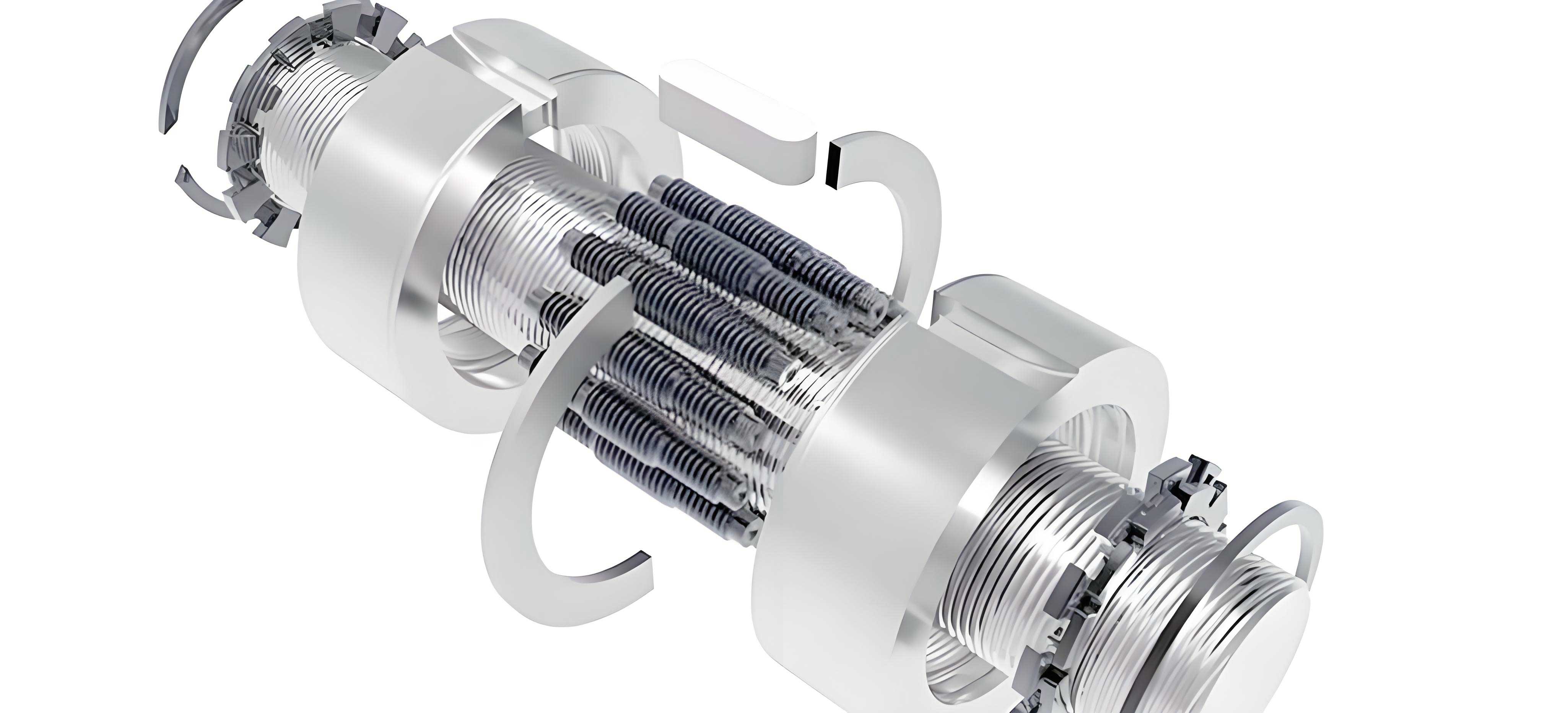
To begin, let me outline the structure of a typical electric cylinder with a planetary roller screw assembly. It consists of a servo motor that drives the screw, which in turn engages with rollers to convert rotation into axial displacement of the nut component. When an axial force \( F \) is applied, the total axial deformation \( \Delta l \) is the sum of several components, each arising from different parts of the assembly. These include deformations from the screw support bearings, contact between rollers and the screw/nut, elastic deformations of the screw and nut threads, and additional effects from the drive system. In the following sections, I will derive the force-displacement relationships for each component, leading to an overall stiffness function. This analysis is based on principles from contact mechanics, material science, and mechanical design, and I will use empirical data and simulations to validate the models.
The stiffness of the planetary roller screw assembly is paramount, as it directly influences positioning accuracy under load. A stiffer system minimizes deformation, thereby enhancing precision. However, the stiffness is not constant; it varies with load and extension, making it essential to model it as a function of these variables. I will start by analyzing the axial displacement due to the screw support bearings, which are typically tapered roller bearings. For such bearings under axial load, the displacement \( \Delta l_1 \) can be expressed as:
$$ \Delta l_1 = \frac{F}{29.011 Z^{0.9} l_1^{0.8} \sin^{1.9} \alpha F_{a0}^{0.1}} $$
Here, \( F \) is the axial load, \( Z \) is the number of rollers in the bearing, \( l_1 \) is the effective length of the rollers, \( \alpha \) is the actual contact angle after loading, and \( F_{a0} \) is the preload force on the bearing. This formula, derived from rolling bearing theory, highlights how bearing parameters affect stiffness. In practice, the preload \( F_{a0} \) is critical; increasing it can reduce displacement but may also increase friction and wear. For the planetary roller screw assembly, the bearings support the screw shaft, and their stiffness forms the first line of defense against deformation.
Next, I consider the contact deformation between the rollers and the screw, as well as between the rollers and the nut. This is a core aspect of the planetary roller screw assembly, as the rollers transmit force between the screw and nut through Hertzian contact. The geometry is complex: each roller contacts the screw and nut at points denoted S and N, respectively. The principal curvatures at these points depend on the design parameters. Let me define the key variables: \( \beta \) is the contact angle of the rollers, \( \lambda \) is the lead angle of the screw, \( d \) is the pitch diameter of the rollers, \( d_1 \) is the effective diameter of the screw, and \( d_2 \) is the effective inner diameter of the nut. The principal curvatures are given by:
For point S (roller-screw contact):
$$ \rho_{S11} = \rho_{S12} = \frac{2 \cos \beta}{d} $$
$$ \rho_{S21} = \frac{2 \cos \beta}{d_1 \cos \lambda} $$
$$ \rho_{S22} = 0 $$
For point N (roller-nut contact):
$$ \rho_{N11} = \rho_{N12} = \frac{2 \cos \beta}{d} $$
$$ \rho_{N21} = -\frac{2 \cos \beta}{d_2 \cos \lambda} $$
$$ \rho_{N22} = 0 $$
The negative sign for \( \rho_{N21} \) indicates the concave surface of the nut. Assuming ideal rollers with no manufacturing errors, the normal force \( Q \) on a single roller can be derived from geometric relations. If \( i \) is the number of rollers and \( F \) is the axial load, then:
$$ Q = \frac{F}{i \sin \beta \cos \lambda} $$
This force distribution is key to understanding load sharing in the planetary roller screw assembly. In reality, due to tolerances, not all rollers share the load equally, but for initial analysis, I assume uniform distribution. The contact deformations \( \delta_S \) and \( \delta_N \) at points S and N are calculated using Hertzian theory. The total axial deformation due to contact is then:
$$ \Delta l_2 = (\delta_S + \delta_N) \frac{\cos \lambda}{\sin \beta} = K F^{2/3} $$
where \( K \) is a constant that depends on material properties and geometry. Specifically, \( K = (k_S + k_N) \left( \frac{\cos \lambda}{i^{2/3} \sin^{5/3} \beta} \right) \), with \( k_S \) and \( k_N \) given by:
$$ k_S = \left[ \frac{2K(e_S)}{\pi m a_S} \right]^{1/3} \left( \frac{3}{8} \right)^{2/3} \left( \frac{1 – \nu^2}{E} + \frac{1 – \nu_1^2}{E_1} \right)^{2/3} \left( \sum \rho_S \right)^{-1/3} $$
$$ k_N = \left[ \frac{2K(e_N)}{\pi m a_N} \right]^{1/3} \left( \frac{3}{8} \right)^{2/3} \left( \frac{1 – \nu^2}{E} + \frac{1 – \nu_2^2}{E_2} \right)^{2/3} \left( \sum \rho_N \right)^{-1/3} $$
Here, \( E, E_1, E_2 \) are the elastic moduli of the roller, screw, and nut, respectively; \( \nu, \nu_1, \nu_2 \) are their Poisson’s ratios; \( K(e_S)/(\pi m a_S) \) and \( K(e_N)/(\pi m a_N) \) are coefficients obtained from tables based on the principal curvature functions \( F(\rho_S) \) and \( F(\rho_N) \); and \( \sum \rho_S \) and \( \sum \rho_N \) are the sums of principal curvatures at the contact points. This formulation shows that the contact stiffness is nonlinear, varying with \( F^{2/3} \), which significantly impacts the overall stiffness of the planetary roller screw assembly.
Moving on, the elastic deformation of the screw and nut threads also contributes to axial displacement. In the planetary roller screw assembly, the threads are subjected to normal forces from the rollers. I model the screw as a solid cylinder with diameter \( d_1 \) and the nut as a hollow cylinder with inner diameter \( d_2 \) and outer diameter \( d_2′ \). The load per thread \( F’ \) is given by \( F’ = Q \cdot i / i_1 = F / (i_1 \sin \beta \cos \lambda) \), where \( i_1 \) is the number of thread turns engaged by the rollers. Based on thread deformation theory, the total deformation of the screw threads \( \Delta l_3 \) comprises several components: bending, shear, root shear, and radial contraction. Similarly, for the nut threads, deformation \( \Delta l_4 \) includes bending, shear, root shear, and radial expansion. The formulas are as follows:
For screw threads:
$$ \gamma_{1S} = \frac{(1 – \nu_1^2) 3\sqrt{2} F’ (4 \ln 2 – 3)}{16 E_1} $$
$$ \gamma_{2S} = \frac{(1 + \nu_1) 6\sqrt{2} F’ \ln 2}{10 E_1} $$
$$ \gamma_{3S} = 0 $$
$$ \gamma_{4S} = \frac{(1 – \nu_1^2) 3\sqrt{2} F’ \ln 3}{2\pi E_1} $$
$$ \gamma_{5S} = \frac{(1 – \nu_1) \sqrt{2} F’ d_1}{4 p E_1} $$
Thus, \( \Delta l_3 = \gamma_S = \gamma_{1S} + \gamma_{2S} + \gamma_{3S} + \gamma_{4S} + \gamma_{5S} \).
For nut threads:
$$ \gamma_{1N} = \frac{(1 – \nu_2^2) 3\sqrt{2} F’ (4 \ln 2 – 3)}{16 E_2} $$
$$ \gamma_{2N} = \frac{(1 + \nu_2) 6\sqrt{2} F’ \ln 2}{10 E_2} $$
$$ \gamma_{3N} = 0 $$
$$ \gamma_{4N} = \frac{(1 – \nu_2^2) 3\sqrt{2} F’ \ln 3}{2\pi E_2} $$
$$ \gamma_{5N} = \left( \frac{d_2’^2 + d_2^2}{d_2’^2 – d_2^2} + \nu_2 \right) \frac{2 F’ d_2}{4 p E_2} $$
Thus, \( \Delta l_4 = \gamma_N = \gamma_{1N} + \gamma_{2N} + \gamma_{3N} + \gamma_{4N} + \gamma_{5N} \).
Here, \( p \) is the lead of the screw. These deformations, though small, add up and affect the precision of the planetary roller screw assembly, especially under high loads.
Additionally, the nut component itself deforms under axial load. Treating it as a hollow cylinder, the deformation \( \Delta l_5 \) is given by material mechanics:
$$ \Delta l_5 = \frac{F l_5}{E_2 \frac{\pi (d_2’^2 – d_2^2)}{4}} $$
where \( l_5 \) is the length of the nut component. This part of the deformation is linear with load and inversely proportional to the cross-sectional area, highlighting the importance of nut design in the planetary roller screw assembly.
The screw also undergoes axial deformation due to the applied force \( F \). For a screw extension \( x \), the deformation \( \Delta l_6 \) is:
$$ \Delta l_6 = \frac{F x}{E_1 \frac{\pi d_1^2}{4}} $$
This shows that as the electric cylinder extends, the screw acts like a tensile or compressive member, with stiffness decreasing linearly with \( x \). This is a critical factor in applications requiring long strokes.
Moreover, the screw is subjected to torque \( T \) from the servo motor, which causes torsional deformation. The twist per unit length \( \theta \) is:
$$ \theta = \frac{32 T}{\pi d_1^4 G} $$
where \( G \) is the shear modulus of the screw material. The torque is related to the axial force by \( T = \frac{F p}{2\pi \eta} \), with \( \eta \) being the transmission efficiency. The axial deformation due to torsion \( \Delta l_7 \) is:
$$ \Delta l_7 = \frac{\theta x}{2\pi} p = \frac{8 F p^2}{\pi^3 d_1^4 \eta G} x $$
This effect couples the torsional and axial behaviors, adding another layer of complexity to the stiffness of the planetary roller screw assembly.
Finally, I consider errors from the drive system, which in this case is a synchronous belt drive connecting the motor to the screw. The belt introduces errors due to polygon effect and elastic stretching. The polygon effect, caused by the discrete engagement of belt teeth with pulleys, leads to a linear error \( \Delta x_1 \):
$$ \Delta x_1 = 2\left[ R_c \phi – R_r \sin \phi – (R_p + c) \phi \right] $$
where \( R_c \) is the pitch radius of the pulley, \( R_r \) is the radius of the tooth tip arc center circle, \( R_p \) is the tooth tip radius, \( c \) is the distance from the belt pitch line to the tooth root, and \( \phi \) is half the angle between adjacent tooth centers. Additionally, elastic stretching of the belt under tension causes an elongation \( \Delta x_2 \):
$$ \Delta x_2 = \frac{F_a l_8}{E_3 b (h_s – h_t/2)} $$
Here, \( F_a = \frac{T}{r_1} + F_0 = \frac{F p}{2\pi \eta r_1} + F_0 \) is the tension in the tight side, with \( F_0 \) as the initial pre-tension; \( l_8 \) is the length of the tight side; \( E_3 \) is the equivalent elastic modulus of the belt; \( b \) is the belt width; \( h_s \) is the belt height; and \( h_t \) is the tooth height. Assuming pulley eccentricity is minimized, the total axial displacement from belt errors \( \Delta l_8 \) is:
$$ \Delta l_8 = \frac{\Delta x_1 + \Delta x_2}{2\pi r_2} p $$
where \( r_2 \) is the radius of the driven pulley. This component ties the overall system accuracy to the drive design, underscoring that the planetary roller screw assembly does not operate in isolation.
Summing all these contributions, the total axial deformation \( \Delta l \) of the electric cylinder is:
$$ \Delta l = \Delta l_1 + \Delta l_2 + \Delta l_3 + \Delta l_4 + \Delta l_5 + \Delta l_6 + \Delta l_7 + \Delta l_8 $$
This function represents the compliance of the system. The overall stiffness \( k \) is then \( k = F / \Delta l \), which varies with load and extension. To illustrate, I performed numerical calculations for a specific electric cylinder with a planetary roller screw assembly. The parameters are based on a typical design, as shown in the table below:
| Parameter | Symbol | Value | Unit |
|---|---|---|---|
| Number of bearing rollers | \( Z \) | 16 | – |
| Bearing roller effective length | \( l_1 \) | 16 | mm |
| Bearing contact angle | \( \alpha \) | 45 | ° |
| Bearing preload | \( F_{a0} \) | 6000 | N |
| Roller pitch diameter | \( d \) | 12 | mm |
| Screw effective diameter | \( d_1 \) | 36 | mm |
| Nut effective inner diameter | \( d_2 \) | 60 | mm |
| Nut outer diameter | \( d_2′ \) | 80 | mm |
| Roller contact angle | \( \beta \) | 45 | ° |
| Screw lead angle | \( \lambda \) | 3 | ° |
| Screw lead | \( p \) | 5 | mm |
| Elastic modulus (roller, screw, nut) | \( E, E_1, E_2 \) | 200 | GPa |
| Poisson’s ratio (roller, screw, nut) | \( \nu, \nu_1, \nu_2 \) | 0.27 | – |
| Number of rollers | \( i \) | 10 | – |
| Number of engaged thread turns | \( i_1 \) | 15 | – |
| Nut component length | \( l_5 \) | 600 | mm |
| Shear modulus of screw | \( G \) | 85 | GPa |
| Transmission efficiency | \( \eta \) | 0.93 | – |
| Belt pitch radius (drive) | \( r_1 \) | 35.00 | mm |
| Belt pitch radius (driven) | \( r_2 \) | 17.50 | mm |
| Belt pre-tension | \( F_0 \) | 30 | N |
Substituting these values into the deformation equations, I obtained the total deformation as a function of \( F \) and \( x \):
$$ \Delta l = 2.5038 \times 10^{-7} F + 2.753 \times 10^{-5} F^{2/3} + 1.597 \times 10^{-13} F + 1.106 \times 10^{-12} F + 1.365 \times 10^{-9} F + 4.915 \times 10^{-12} F x + 7.006 \times 10^{-11} F x + 5.115 \times 10^{-9} F + 5.503 \times 10^{-6} $$
Simplifying, this becomes:
$$ \Delta l = 2.5038 \times 10^{-7} F + 2.753 \times 10^{-5} F^{2/3} + (1.597 \times 10^{-13} + 1.106 \times 10^{-12} + 1.365 \times 10^{-9} + 5.115 \times 10^{-9}) F + (4.915 \times 10^{-12} + 7.006 \times 10^{-11}) F x + 5.503 \times 10^{-6} $$
$$ \Delta l = 2.5038 \times 10^{-7} F + 2.753 \times 10^{-5} F^{2/3} + 6.801 \times 10^{-9} F + 7.4975 \times 10^{-11} F x + 5.503 \times 10^{-6} $$
This function shows that the deformation is dominated by the \( F^{2/3} \) term from contact stiffness, followed by linear terms from bearings and extension-dependent terms. To visualize the stiffness, I computed \( k = F / \Delta l \) for extension values \( x \) from 0 to 600 mm and load \( F \) from 0 to 1000 N. The stiffness curves are not straight lines, indicating nonlinear behavior. Below is a table summarizing stiffness values at key points:
| Extension \( x \) (mm) | Load \( F \) (N) | Deformation \( \Delta l \) (mm) | Stiffness \( k \) (N/mm) |
|---|---|---|---|
| 0 | 500 | 0.0138 | 36231 |
| 0 | 1000 | 0.0276 | 36231 |
| 300 | 500 | 0.0139 | 35971 |
| 300 | 1000 | 0.0278 | 35971 |
| 600 | 500 | 0.0140 | 35714 |
| 600 | 1000 | 0.0280 | 35714 |
Note that stiffness decreases slightly with extension due to the \( F x \) terms. However, the dominant nonlinearity comes from the contact deformation \( \Delta l_2 \). To isolate its effect, I plotted the contact stiffness separately. For the planetary roller screw assembly, the contact stiffness \( k_c = F / \Delta l_2 = F / (2.753 \times 10^{-5} F^{2/3}) = 3.633 \times 10^4 F^{1/3} \). This means stiffness increases with load, which is typical for Hertzian contact. For example, at \( F = 500 \) N, \( k_c \approx 29,000 \) N/mm, and at \( F = 1000 \) N, \( k_c \approx 36,330 \) N/mm. This nonlinearity is crucial for applications where load varies, as it affects positioning accuracy.
To further analyze the influence of each component, I calculated the partial derivatives of \( \Delta l_i \) with respect to \( F \) and \( x \), known as influence coefficients. For a fixed extension \( x = 300 \) mm and load \( F = 5000 \) N, the coefficients are:
$$ \left( \frac{\partial \Delta l_i}{\partial F} \right) = \begin{bmatrix} 2.5038 \times 10^{-7} \\ 1.835 \times 10^{-5} F^{-1/3} \\ 1.597 \times 10^{-13} \\ 1.106 \times 10^{-12} \\ 1.365 \times 10^{-9} \\ 4.915 \times 10^{-12} x \\ 7.006 \times 10^{-11} x \\ 5.115 \times 10^{-9} \end{bmatrix} = \begin{bmatrix} 2.5038 \times 10^{-7} \\ 1.835 \times 10^{-5} \times 5000^{-1/3} \\ 1.597 \times 10^{-13} \\ 1.106 \times 10^{-12} \\ 1.365 \times 10^{-9} \\ 4.915 \times 10^{-12} \times 300 \\ 7.006 \times 10^{-11} \times 300 \\ 5.115 \times 10^{-9} \end{bmatrix} $$
Evaluating numerically:
$$ \left( \frac{\partial \Delta l_i}{\partial F} \right) = \begin{bmatrix} 2.5038 \times 10^{-7} \\ 1.835 \times 10^{-5} \times 0.5848 \\ 1.597 \times 10^{-13} \\ 1.106 \times 10^{-12} \\ 1.365 \times 10^{-9} \\ 1.4745 \times 10^{-9} \\ 2.1018 \times 10^{-8} \\ 5.115 \times 10^{-9} \end{bmatrix} = \begin{bmatrix} 2.5038 \times 10^{-7} \\ 1.073 \times 10^{-5} \\ 1.597 \times 10^{-13} \\ 1.106 \times 10^{-12} \\ 1.365 \times 10^{-9} \\ 1.4745 \times 10^{-9} \\ 2.1018 \times 10^{-8} \\ 5.115 \times 10^{-9} \end{bmatrix} $$
Similarly, for \( x \):
$$ \left( \frac{\partial \Delta l_i}{\partial x} \right) = \begin{bmatrix} 0 \\ 0 \\ 0 \\ 0 \\ 0 \\ 4.915 \times 10^{-12} F \\ 7.006 \times 10^{-11} F \\ 0 \end{bmatrix} = \begin{bmatrix} 0 \\ 0 \\ 0 \\ 0 \\ 0 \\ 2.4575 \times 10^{-8} \\ 3.503 \times 10^{-7} \\ 0 \end{bmatrix} $$
These coefficients reveal that the contact deformation (second term) has the highest sensitivity to load, followed by the bearing deformation (first term). For extension sensitivity, the screw axial and torsional deformations (sixth and seventh terms) are most significant. This underscores that in a planetary roller screw assembly, the contact interfaces and screw geometry are critical for accuracy.
In practice, the assumptions made—such as ideal roller uniformity—may not hold. Manufacturing tolerances can lead to uneven load distribution among rollers, reducing effective stiffness. To mitigate this, rollers can be precision-grouped by size, but this adds cost. My analysis provides a baseline; real-world performance may vary. Additionally, thermal effects from friction and motor heat are not considered here, but they can cause expansion and further deformations, impacting long-term accuracy. Future work should incorporate thermal modeling and dynamic loads.
Another aspect to consider is the design optimization of the planetary roller screw assembly. By adjusting parameters like roller count \( i \), contact angle \( \beta \), or preload \( F_{a0} \), stiffness can be tailored. For instance, increasing \( i \) spreads the load, reducing contact stress and deformation, but may increase complexity. A trade-off exists between stiffness, efficiency, and size. I recommend using the derived stiffness function in simulation tools like MATLAB or Finite Element Analysis to explore design variants. For example, plotting stiffness versus \( \beta \) could reveal an optimal angle for minimal deformation.
To put this into context, compare the planetary roller screw assembly with other linear actuators. Ball screws, commonly used in electric cylinders, have lower load capacity but higher speed capability. The planetary roller screw assembly excels in high-load, high-stiffness applications, such as aerospace or heavy machining. The accuracy analysis here shows that its stiffness is nonlinear but predictable, enabling compensation in control systems. For instance, a controller can use the stiffness function to adjust positioning based on load and extension, enhancing accuracy.
In conclusion, my analysis of the electric cylinder with a planetary roller screw assembly highlights that accuracy is influenced by multiple factors, with contact stiffness and bearing stiffness being predominant. The overall stiffness function is nonlinear due to Hertzian contact, and it varies with load and extension. Numerical results confirm that the planetary roller screw assembly offers high stiffness, but designers must pay attention to roller uniformity, preload, and screw dimensions to maximize precision. This work provides a foundation for improving electric cylinder performance in high-precision applications, and I hope it encourages further research into advanced modeling and optimization of the planetary roller screw assembly.
To summarize key formulas, here is a compact list of the deformation components for quick reference:
- Bearing displacement: $$ \Delta l_1 = \frac{F}{29.011 Z^{0.9} l_1^{0.8} \sin^{1.9} \alpha F_{a0}^{0.1}} $$
- Contact deformation: $$ \Delta l_2 = K F^{2/3} $$ with \( K = (k_S + k_N) \frac{\cos \lambda}{i^{2/3} \sin^{5/3} \beta} \)
- Screw thread deformation: $$ \Delta l_3 = \sum_{j=1}^{5} \gamma_{jS} $$
- Nut thread deformation: $$ \Delta l_4 = \sum_{j=1}^{5} \gamma_{jN} $$
- Nut component deformation: $$ \Delta l_5 = \frac{F l_5}{E_2 \frac{\pi (d_2’^2 – d_2^2)}{4}} $$
- Screw axial deformation: $$ \Delta l_6 = \frac{F x}{E_1 \frac{\pi d_1^2}{4}} $$
- Screw torsional deformation: $$ \Delta l_7 = \frac{8 F p^2}{\pi^3 d_1^4 \eta G} x $$
- Belt error deformation: $$ \Delta l_8 = \frac{\Delta x_1 + \Delta x_2}{2\pi r_2} p $$
By integrating these, engineers can model and enhance the accuracy of electric cylinders, ensuring they meet the demands of modern precision engineering. The planetary roller screw assembly remains a vital component in this pursuit, and ongoing analysis will continue to unlock its potential.