
The pursuit of high precision and reliability in power transmission systems has been a central focus of my research, particularly in applications like robotics, aerospace mechanisms, and precision instrumentation. Among various solutions, the strain wave gear, also known as a harmonic drive, stands out for its exceptional advantages: compact size, high single-stage reduction ratio, zero-backlash operation, and high torque capacity. However, achieving and maintaining its renowned positional accuracy over a long operational life presents significant challenges. The inherent elastic deformation of its key component—the flexspline—and the inevitable wear at critical interfaces introduce dynamic errors that static error models fail to capture. My investigation aims to bridge this gap by developing a comprehensive transmission error model that integrates both static manufacturing/assembly variances and the dynamic effects of wear and deformation. Subsequently, I perform a time-variant reliability analysis of the transmission accuracy and propose a reliability-based optimization design to ensure performance longevity.
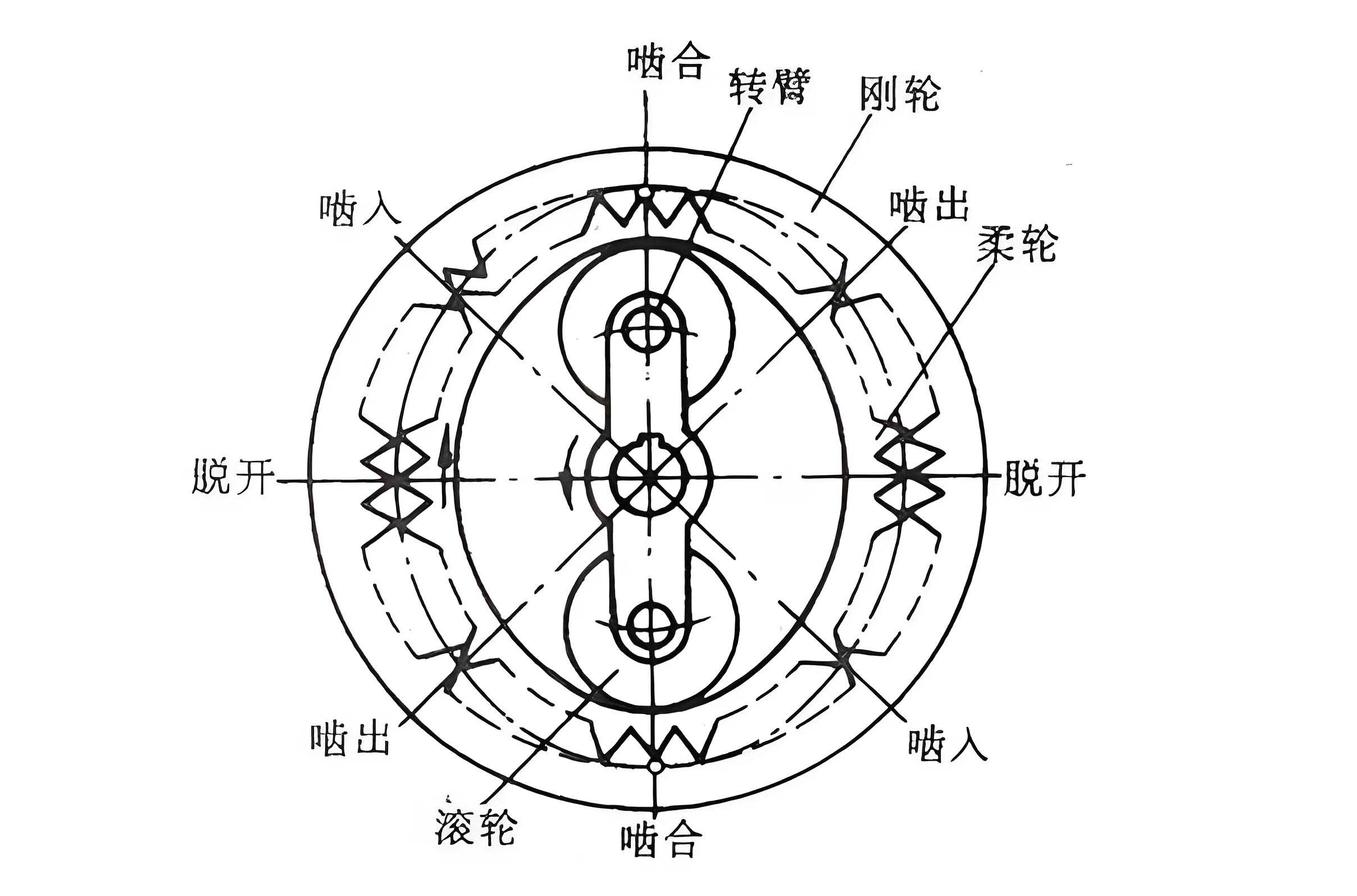
1. Comprehensive Transmission Error Analysis for the Strain Wave Gear
The fundamental operation of a strain wave gear relies on the controlled elastic deformation of a thin-walled flexspline by an elliptical wave generator, causing it to mesh with a rigid circular spline. The kinematic error, defined as the deviation between the theoretical and actual output rotation, stems from multiple sources. My analysis categorizes these into static errors from manufacturing and assembly, and dynamic errors arising from operational factors.
The primary static errors include the manufacturing inaccuracies of the circular spline and flexspline, such as cumulative pitch error \((\Delta F_p)\) and adjacent pitch error \((\Delta f_f)\), as well as assembly-induced eccentricities from radial runouts and fitting clearances at mounting interfaces. The dynamic errors are predominantly caused by the wear at the interface between the flexspline’s inner wall and the wave generator bearing’s outer race, and the time-varying deformation of the flexspline under load and speed.
I formulate the total transmission error by statistically combining these independent error sources. The equivalent linear error along the line of action can be expressed as the root-sum-square of individual error components. This static error \(\Delta x_m\) is given by:
$$ \Delta x_m = \frac{1}{2 \cos \alpha_n} \sqrt{\Delta F_{p1}^2 + \Delta F_{p2}^2 + \Delta f_{f1}^2 + \Delta f_{f2}^2 + \sum e_j^2} $$
where \(\alpha_n\) is the nominal pressure angle, subscripts 1 and 2 denote the circular spline and flexspline respectively, and \(e_j\) represents various assembly clearance and runout errors.
To account for dynamics, I introduce two key additions: a wear-induced radial error \(e_V(T, v, t)\) and a deformation-induced radial displacement error \(e_B(T, v)\). The wear error effectively increases the radial clearance within the wave generator assembly over time \(t\), under operational load \(T\) and input speed \(v\). The deformation error represents the additional radial displacement of the flexspline cup’s rim under operational conditions, beyond its nominal pre-deformation by the wave generator. Incorporating these, the refined total equivalent error becomes:
$$ \Delta x_{total} = \frac{1}{2 \cos \alpha_n} \sqrt{\Delta F_{p1}^2 + \Delta F_{p2}^2 + \Delta f_{f1}^2 + \Delta f_{f2}^2 + \sum e_i^2 + \left(e_{WG1} + V(T,v,t)\right)^2 + \left(e_{WG2} + B(T,v)\right)^2} $$
Here, \(e_{WG1}\) and \(e_{WG2}\) are static errors associated with the wave generator’s non-rotating and rotating eccentricities, respectively. \(V(T,v,t)\) is the dynamic wear depth, and \(B(T,v)\) is the dynamic radial displacement due to flexspline deformation. Finally, this linear error is converted into an angular error at the output shaft \(\Delta \theta_{out}\) for practical assessment:
$$ \Delta \theta_{out} = k_c \times \Delta x_{total} $$
$$ \text{where } k_c = \frac{k_b}{\sqrt{N}} \times \frac{206.4}{d_1} $$
\(k_b\) is a correlation coefficient, \(N\) is the number of simultaneously engaged tooth pairs, and \(d_1\) is the pitch diameter of the driven gear. This model forms the foundation for the subsequent reliability analysis of the strain wave gear system.
2. Modeling of Dynamic Wear and Flexspline Deformation
Accurately characterizing the dynamic factors \(V(T,v,t)\) and \(B(T,v)\) is paramount for a realistic reliability assessment. My approach combines physical modeling with data-driven techniques to capture their complex, non-linear behavior.
2.1 Bayesian-Calibrated Dynamic Wear Model
The wear between the flexspline (typically made of 40Cr steel) and the wave generator bearing outer race (GCr15 steel) operates in a mixed lubrication regime, leading to adhesive and abrasive wear. An established empirical model for adhesive wear rate \(\phi\) under mixed lubrication is:
$$ \phi = \frac{dV}{dt} = \frac{2 k_e k_s W f}{3 \sigma_s (f_B – f_E)} \left(1 + 3(f – f_E)^2\right)^{1/2} $$
where \(k_e, k_s\) are coefficients, \(W\) is load, \(\sigma_s\) is yield stress, and \(f_B, f_E, f\) are friction coefficients for boundary, full-film, and mixed lubrication states, respectively.
However, this model alone does not fully account for the impact loading and complex stress state in an operating strain wave gear. To calibrate it with reality, I employ a Bayesian framework. The corrected wear model \(V_{re}\) is expressed as:
$$ V_{re}(T’, v’, t’) = V_{or}(T’, v’, t’) + \Delta V^*(T’, v’, t’) + \varepsilon_V $$
Here, \(V_{or}\) is the wear volume from the empirical model integrated over time, \(\Delta V^*\) is a model discrepancy term, and \(\varepsilon_V\) is a random error \(\varepsilon_V \sim N(0.09, 0.03^2)\). The discrepancy term \(\Delta V^*\) is modeled using Gaussian Process (GP) regression trained on experimental wear data. I conducted accelerated wear tests on a specific strain wave gear model under various load-speed-time profiles, as summarized below:
| Test ID | Output Load, T (N·m) | Input Speed, v (r/min) | Duration, t (h) | Measured Wear, V (μm) |
|---|---|---|---|---|
| 1 | 17.5 | 300 | 550 | 2.98 |
| 2 | 38.0 | 100 | 550 | 3.85 |
| 3 | 25.0 | 300 | 1200 | 5.34 |
| 4 | 17.5 | 100 | 1750 | 5.09 |
| 5 | 25.0 | 500 | 1750 | 7.12 |
| 6 | 38.0 | 300 | 2150 | 9.83 |
| 7 | 25.0 | 300 | 3250 | 10.02 |
| 8 | 38.0 | 500 | 3250 | 11.17 |
| 9 | 17.5 | 300 | 3650 | 9.79 |
The GP model, trained on this data, predicts the discrepancy for any given operational condition \((T’, v’, t’)\). The final wear model thus synergizes physics and data, providing more accurate predictions, as validated against separate test data where measurements fell within the model’s 95% confidence interval.
2.2 Data-Driven Flexspline Deformation Model
The radial deformation of the flexspline cup’s open end is a critical source of high-frequency transmission error. This deformation is not constant; it varies with load and speed due to dynamic effects like centrifugal stiffening and changing mesh stiffness. To quantify this, I built a test rig to measure the maximum radial displacement \(B\) of the flexspline rim using a laser displacement sensor under various operational parameters.
Given the cost and complexity of exhaustive testing, I again employed GP regression to build a predictive model \(B_{pre}(T’, v’)\). The model was trained on experimental data from a designed set of load-speed combinations. The predictive performance was excellent, with validation data points lying well within the 95% prediction confidence band. This model allows me to estimate the dynamic deformation component \(B(T,v)\) for any load and speed within the trained range, effectively integrating this complex effect into the overall error model of the strain wave gear.
3. Time-Variant Reliability Analysis of Transmission Accuracy
With the comprehensive error model established, I can now analyze the reliability of the strain wave gear’s transmission accuracy. Reliability, in this context, is defined as the probability that the output angular error \(\Delta \theta_{out}\) remains below a specified allowable limit \(\theta_{al}\) throughout a required service time. This is a time-variant problem because wear \(V(T,v,t)\) is a function of time.
The performance function \(g\) for reliability analysis is:
$$ g(\mathbf{a}, \theta_{al}) = \theta_{al} – \Delta \theta_{out}(\mathbf{a}) $$
where \(\mathbf{a} = (T, v, t, \Delta F_{p1}, \Delta F_{p2}, …)\) is the vector of all random variables (operational parameters and error terms). Failure occurs when \(g < 0\). The time-variant reliability \(R(t)\) is:
$$ R(t) = P(g(\mathbf{a}, \theta_{al}) > 0 \ \forall \ \tau \in [0, t]) \approx 1 – P_f(t) $$
where \(P_f(t)\) is the probability of failure by time \(t\). All static error parameters are treated as independent normal random variables. Their distribution parameters (mean and standard deviation) are derived from manufacturing tolerances, as exemplified below for a specific strain wave gear design.
| Error Parameter | Symbol | Tolerance (μm) | Std. Dev. (μm) |
|---|---|---|---|
| Circular Spline Adjacent Pitch Error | \(\Delta f_{f1}\) | 16 | 2.67 |
| Flexspline Adjacent Pitch Error | \(\Delta f_{f2}\) | 16 | 2.67 |
| Circular Spline Cumulative Pitch Error | \(\Delta F_{p1}\) | 36 | 6.00 |
| Flexspline Cumulative Pitch Error | \(\Delta F_{p2}\) | 36 | 6.00 |
| Radial Runout (Circular Spline Mount) | \(e_{CS11}\) | 12 | 2.00 |
| Fitting Clearance (Circular Spline) | \(e_{CS12}\) | 45 | 7.50 |
| Fitting Clearance (Flexspline-Output Shaft) | \(e_{FS11}\) | 21 | 3.50 |
| Radial Runout (Output Shaft) | \(e_{FS12}\) | 12 | 2.00 |
| Wave Generator Bearing Radial Clearance | \(e_{WG11}\) | 20 | 3.33 |
| Wave Generator Bearing Radial Runout | \(e_{WG12}\) | 25 | 4.17 |
| Clearance (Cam-Bearing) | \(e_{WG21}\) | 15 | 2.50 |
| Clearance (Bearing-Flexspline) | \(e_{WG22}\) | 20 | 3.33 |
Evaluating the reliability directly via Monte Carlo Simulation (MCS) on the high-fidelity error model (which includes the GP wear and deformation models) is computationally expensive. To achieve efficiency, I construct a surrogate model. I use Latin Hypercube Sampling (LHS) to select a set of training points over the space of input variables, including time slices. For each sampled point \((T, v, t)\) and a random draw of static errors, I compute the total error \(\Delta \theta_{out}\) using the full physics-data model.
I then employ Kriging interpolation to build a fast-running surrogate model \(J(\mathbf{w})\) that approximates the output error for any input vector \(\mathbf{w} = (T_x, v_x, t_x, …)\). The reliability at a given time is then efficiently computed by performing MCS on this Kriging surrogate model.
For a case study with fixed operational parameters (T=17.5 N·m, v=100 r/min) and an allowable error, the reliability degrades over time as wear accumulates. The analysis shows reliability remains high initially but experiences a more significant decline as operational hours increase, dropping to approximately 91.17% at 3,000 hours for the initial design configuration. This highlights the necessity of considering wear in the long-term reliability assessment of a strain wave gear.
4. Reliability-Based Optimization Design
The initial reliability analysis revealed a potential for improvement. My goal is to optimize the design tolerances to enhance the long-term transmission accuracy reliability without incurring excessive manufacturing cost. This is formulated as a reliability-based design optimization (RBDO) problem.
4.1 Sensitivity Analysis and Design Variables
To reduce the problem dimension, I first conducted a sensitivity analysis on the static error parameters with respect to the output transmission error. The normalized sensitivity \(\Delta s_i\) is calculated as:
$$ s_i = \frac{\partial \Delta \theta_{out}}{\partial \Delta e_i}, \quad \Delta s_i = \frac{s_i}{\sum_{i=1}^{12} s_i} $$
The results indicated that the cumulative pitch errors (\(\Delta F_{p1}, \Delta F_{p2}\)) and a major assembly clearance (\(e_{CS12}\)) were the most significant contributors. Several parameters like certain adjacent pitch errors and runouts had minor influence. I selected the three most sensitive and five least sensitive parameters as design variables for optimization, allowing the tolerances on critical items to be tightened while possibly relaxing others to save cost.
4.2 Optimization Problem Formulation
The RBDO problem is formulated with the objective to minimize total manufacturing cost \(C(\Delta \mathbf{e}’)\) subject to reliability and wear constraints.
Objective Function (Minimize Cost):
The cost for machining a tolerance \(Z_{e’_i}\) is modeled by tolerance-cost functions. For size (fit) tolerance \(C_1\), position tolerance \(C_2\), and runout tolerance \(C_3\):
$$ C_1(Z_{e’_i}) = a_{e’} – b_{e’} Z_{e’_i} + \frac{e_{e’}}{c_{e’} \cdot Z_{e’_i} + d_{e’}} $$
$$ C_2(Z_{e’_i}) = f_{e’} e^{-g_{e’} Z_{e’_i}} + h_{e’} Z_{e’_i}^{-l_{e’}} $$
$$ C_3(Z_{e’_i}) = m_{e’} e^{-s_{e’} Z_{e’_i}} $$
The total cost is the sum of individual cost items: \(C(\Delta \mathbf{e}’) = \sum_{i=1}^{8} k_j C_j(e’_i)\), where \(k_j\) selects the appropriate cost function type.
Constraints:
- Reliability Constraint: The reliability at the target mission time (e.g., t=3000 hours) must meet or exceed a required threshold \(P_{re}\).
$$ P(\Delta \mathbf{e}’)(T, v, t) \ge P_{re} $$ - Wear Constraint: The predicted maximum wear at end-of-life should be less than an allowable limit \(V_{pre}\).
$$ V(\Delta \mathbf{e}’, (T, v, t)) \le V_{pre} $$ - Bound Constraints: Tolerances must remain within feasible manufacturing limits.
$$ \delta_{min} \le e’_i \le \delta_{max} $$
4.3 Optimization Results and Discussion
I solved this nonlinear constrained optimization problem using the Sequential Quadratic Programming (SQP) algorithm. The table below compares the initial and optimized tolerance values for the selected design variables.
| Design Variable (Tolerance) | Initial Value (μm) | Optimized Value (μm) |
|---|---|---|
| \(\Delta F_{p1}\) (Circular Spline Cum. Pitch) | 36.0 | 32.4 |
| \(\Delta F_{p2}\) (Flexspline Cum. Pitch) | 36.0 | 31.3 |
| \(e_{CS12}\) (Major Assembly Clearance) | 45.0 | 38.7 |
| \(\Delta f_{f1}\) (Circular Spline Adj. Pitch) | 16.0 | 16.7 |
| \(\Delta f_{f2}\) (Flexspline Adj. Pitch) | 16.0 | 16.7 |
| \(e_{CS11}\) (Radial Runout) | 12.0 | 13.3 |
| \(e_{FS12}\) (Output Shaft Runout) | 12.0 | 13.2 |
| \(e_{WG21}\) (Cam-Bearing Clearance) | 15.0 | 15.4 |
The optimization intelligently tightened the critical tolerances (\(\Delta F_{p1}, \Delta F_{p2}, e_{CS12}\)) while slightly relaxing some less sensitive ones (\(\Delta f_{f1}, \Delta f_{f2}, e_{CS11}, etc.\)). The net effect was a marginal increase in total manufacturing cost of only 1.70%. However, the impact on reliability was profound. Re-evaluating the time-variant reliability with the optimized tolerances showed a significant improvement. At the 3,000-hour mark, the transmission accuracy reliability rose to 99.02%, an increase of 7.85 percentage points from the initial 91.17%.
This outcome validates the efficacy of the proposed framework. By systematically integrating dynamic wear and deformation models into a comprehensive error analysis, performing a time-variant reliability assessment, and executing a cost-constrained reliability optimization, I demonstrated a practical methodology to significantly enhance the long-term performance robustness of a strain wave gear. This approach ensures that the high precision expected from these sophisticated mechanisms is maintained throughout their intended service life, which is crucial for their application in demanding fields like robotics and aerospace.