
In this work, I study the accurate modeling, tooth-surface correction, and contact performance of the spiral bevel gear from a first-person research perspective. A spiral bevel gear is widely used in intersecting-axis and offset-axis power transmission because it can provide a large transmission ratio, smooth motion, and strong load capacity. However, its tooth surface is a complex spatial surface. The design, manufacturing correction, and meshing analysis of a spiral bevel gear are therefore strongly coupled. I focus on three linked problems: how to construct a truly accurate geometric model, how to correct machining errors using general machine-tool settings, and how to evaluate static and dynamic meshing behavior using finite element analysis.
I first explain why a conventional conjugate-surface design of a spiral bevel gear often produces only an approximate spherical involute. I then derive a spherical-involute-based mathematical model and build a precise three-dimensional solid model. Next, I propose an ease-off-based correction method using universal generation machine settings. Finally, I build high-quality finite element models and analyze contact stress, bending stress, contact path, transmission error, speed effects, acceleration-time effects, and load effects. The results provide practical guidance for the design, manufacturing, vibration reduction, and noise reduction of a spiral bevel gear transmission.
1. Background and Motivation for Spiral Bevel Gear Research
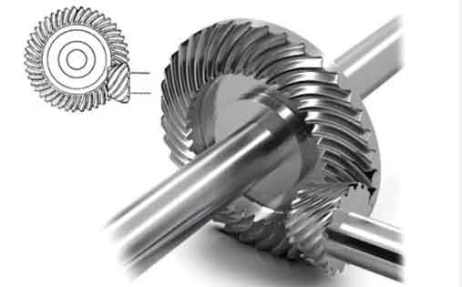
A spiral bevel gear transmits motion between shafts that usually intersect at a right angle or at another fixed angle. Because the teeth are curved along the face width, the contact ratio is larger than that of a straight bevel gear, and the motion is smoother. For this reason, the spiral bevel gear is common in aviation, aerospace, marine equipment, automobiles, machine tools, construction machinery, and mining machinery. Despite these advantages, the spiral bevel gear is difficult to design and manufacture accurately. Its tooth surface is generated by a complex relative motion between a cutter and a workpiece. Small changes in machine settings can produce visible changes in the contact pattern and transmission error.
In the traditional design framework, the conjugate-surface principle is used as the theoretical basis. The condition for two conjugate surfaces can be written as
$$ \mathbf{r}_2=\mathbf{r}_1+\mathbf{m}, \qquad \mathbf{n}_2=\mathbf{n}_1, $$
where the two surfaces are in contact and share a common tangent plane. The meshing equation is
$$ \mathbf{v}_{12}\cdot\mathbf{n}=0, $$
where the relative velocity is perpendicular to the common normal. This principle is elegant and powerful, but when it is applied to a spiral bevel gear through a particular generation motion, the resulting tooth profile is often not an exact spherical involute. It is an approximation. This introduces a principle error that must later be compensated by modification, adjustment, or trial cutting. Such compensation increases cost, reduces efficiency, and makes the design less repeatable.
I therefore adopt the spherical involute as the fundamental tooth profile for the spiral bevel gear. During meshing, the contact point of a bevel gear lies on a sphere whose center is the cone apex. The exact tooth profile should therefore be a spherical curve, not a planar approximation. A spherical involute profile can improve stress distribution, reduce noise, reduce transmission error, and stabilize the instantaneous transmission ratio. Table 1 summarizes the comparison between the approximate conjugate design and the spherical involute design that I use.
| Item | Approximate Conjugate Design | Spherical Involute Design |
|---|---|---|
| Theoretical basis | Conjugate surfaces generated by a specific machine motion | Exact spherical involute on a sphere centered at the cone apex |
| Profile accuracy | Approximate spherical involute | Exact spherical involute within the chosen mathematical representation |
| Principle error | Present and often non-negligible | Reduced or eliminated at the profile-definition level |
| Manufacturing correction | Often relies on trial cutting and empirical adjustment | Can be combined with systematic ease-off correction |
| Transmission quality | May show unstable ratio, edge contact, and noise | Promotes smoother meshing and more uniform stress |
| Design repeatability | Depends on machine and cutter specifics | More suitable for parameterization and digital design |
2. Spherical Involute Geometry for the Spiral Bevel Gear
I consider a cone gear pair in correct mesh. The two pitch cones are tangent and roll without slipping, and their apexes coincide. The distance from the meshing point to the common apex remains constant. Therefore, the path of the contact point is a spherical curve. To derive the spherical involute, I imagine a plane tangent to a base cone. When this plane rolls without slipping on the base cone, a point fixed in the plane traces a spherical involute on the sphere centered at the cone apex.
Let the spherical involute point be denoted by K. Let the base cone angle be \(\delta_b\), and let the cone angle of point K be \(\delta_k\). In a spherical coordinate system whose origin is the cone apex, the point can be written as
$$ K=(R,\delta_k,\beta), $$
where \(R\) is the spherical radius and \(\beta\) is the polar angle. From the geometry of the rolling plane and the base cone, I obtain
$$ OP = OK\frac{\cos\delta_k}{\cos\delta_b}. $$
The arc length relationship on the sphere gives
$$ \widehat{K_0K}=\widehat{K_0N}=OK\arccos(\cos\delta_k\cos\delta_b). $$
The spherical angle relation gives
$$ \angle K_0ON=\frac{\arccos(\cos\delta_k\cos\delta_b)}{\sin\delta_b}. $$
I also have
$$ \angle K_0OK=\arctan\frac{\tan\delta_b}{\tan\delta_k}. $$
Therefore, the polar angle of the spherical involute is
$$ \beta=\frac{\arccos(\cos\delta_k\cos\delta_b)}{\sin\delta_b}-\arctan\frac{\tan\delta_b}{\tan\delta_k}. $$
This equation is the core of the exact profile. The spherical involute point is then
$$ \mathbf{K}=(R,\delta_k,\beta). $$
For a spiral bevel gear, the working part of the tooth profile follows this spherical involute, while the addendum, dedendum, and fillet are connected to it. I divide the complete tooth profile into four parts: the addendum arc, the working profile, the fillet, and the dedendum arc. Table 2 lists these components and their roles.
| Profile Component | Symbol | Geometric Role | Meshing Role |
|---|---|---|---|
| Addendum arc | \(h_1\) | Connects the top land to the working profile | Does not carry the main contact load |
| Working profile | \(h_2\) | Exact spherical involute | Main active contact surface |
| Fillet | \(h_3\) | Connects the working profile to the dedendum | Affects root bending stress |
| Dedendum arc | \(h_4\) | Forms the bottom clearance region | Does not participate in normal meshing |
3. Mathematical Formulation of the Spiral Bevel Gear Tooth Surface
I introduce a parameter \(t\in[0,1]\) so that each profile curve can be swept smoothly. At the large end, the working profile is a spherical involute. Its equation is
$$ \mathbf{h}_2(t)=\left(R,\ \delta_a t+\delta_f(1-t),\ \beta\right), $$
where \(\delta_a\) is the addendum cone angle and \(\delta_f\) is the dedendum cone angle. The opposite working profile is obtained by a rotation of the tooth thickness angle:
$$ \varphi_k=\beta-\frac{360^\circ}{z}-\phi_b, $$
where \(z\) is the number of teeth and \(\phi_b\) is the tooth thickness angle. For the addendum arc at the large end, I write
$$ \mathbf{h}_1(t)=\left(R,\ \delta_a,\ \beta+\delta_{as}t\right), $$
where \(\delta_{as}\) is the addendum thickness angle. For the dedendum arc at the large end, I write
$$ \mathbf{h}_4(t)=\left(R,\ \delta_f,\ \beta+\delta_{fs}t\right), $$
where \(\delta_{fs}\) is the dedendum thickness angle. The opposite dedendum arc is
$$ \varphi_k=\beta-\frac{360^\circ}{z}-\phi_f, $$
where \(\phi_f\) is the dedendum thickness angle.
The fillet is generated by the cutter tip or cutter corner. Its exact expression is not convenient for direct use, so I use an approximate but controlled formulation. When the base radius is not greater than the root radius, the fillet radius can be taken as
$$ R_f=0.3m_{ne}, $$
where \(m_{ne}\) is the normal module. When the base radius is greater than the root radius, the fillet starts at the intersection of the base circle and the working profile and ends at the intersection of the base circle and the dedendum arc. I then use an arc whose radius satisfies
$$ R_f\le r_{\max}, $$
where \(r_{\max}\) is the maximum cutter tip radius.
The lead line is chosen as the guiding curve for sweeping the profile. If the midpoint of the lead line has spherical radius \(R_P\) and spiral angle \(\beta_P\), and if a general point on the lead line has radius \(R’\) and spiral angle \(\beta’\), then the lead-line condition can be written as
$$ f(R’,\beta’)=0. $$
A convenient form is
$$ \sin\beta’=\frac{r_0^2+R’^2-R_P^2}{2r_0R’}, $$
where \(r_0\) is the cutter radius. The small end is obtained by reducing the spherical radius by the face width \(B\). Its profile is
$$ \mathbf{h}_s(t)=\left(R-B,\ \theta_k,\ \varphi_k\pm\Delta\phi\right), $$
where the spherical offset is
$$ \Delta\phi=\frac{\Delta\epsilon}{\sin\delta}. $$
The angular change along the lead line is
$$ \Delta\epsilon=\arcsin\left(\frac{r_0(\cos\beta_a-\cos\beta_f)}{S_d}\right), $$
where \(S_d\) is the radial cutter position. Table 3 summarizes the key mathematical curves used in the exact spiral bevel gear model.
| Curve | Mathematical Description | Key Parameters |
|---|---|---|
| Working profile \(h_2\) | Spherical involute | \(R,\delta_a,\delta_f,\delta_b,\beta\) |
| Addendum arc \(h_1\) | Arc at addendum cone angle | \(\delta_a,\delta_{as}\) |
| Dedendum arc \(h_4\) | Arc at dedendum cone angle | \(\delta_f,\delta_{fs}\) |
| Fillet \(h_3\) | Controlled fillet radius | \(m_{ne},r_{\max},r_b,r_f\) |
| Lead line | Spiral curve along face width | \(r_0,R_P,\beta_P,S_d\) |
| Small-end profile | Offset large-end profile | \(B,\Delta\phi,\delta\) |
4. Construction of the Accurate Spiral Bevel Gear Solid Model
I build the solid model by sweeping the large-end and small-end profiles along the lead line. First, I construct the base cone from the computed base cone angle and cone distance. Second, I create the large-end and small-end profile curves from the parametric equations above. Third, I create the lead line as the guiding curve. Fourth, I sweep the profile curves along the lead line to form one tooth. Fifth, I pattern the single tooth around the gear axis. Finally, I trim and unite the tooth bodies with the gear blank.
The steps I use are listed in Table 4. This sequence is important because the spiral bevel gear surface is not a simple extruded or revolved surface. A small error in the lead line or in the profile curve can propagate into the entire tooth surface.
| Step | Operation | Purpose |
|---|---|---|
| 1 | Construct base cone | Define the spherical reference surface |
| 2 | Create large-end profile | Define the exact spherical involute tooth shape |
| 3 | Create small-end profile | Define the profile at the other side of the face width |
| 4 | Create lead line | Define the spiral direction along the face width |
| 5 | Sweep profiles | Generate a single spiral bevel gear tooth |
| 6 | Pattern and unite | Generate the complete spiral bevel gear solid |
After the pinion and gear are modeled, I assemble them in the three-dimensional environment. I set the shaft angle, mounting distance, and axial positions using reference planes and axes. I then adjust the angular position so that the teeth do not interfere at the initial contact position. The design parameters used in my model are given in Table 5.
| Parameter | Gear | Pinion |
|---|---|---|
| Number of teeth | 43 | 11 |
| Module (mm) | 4.65 | 4.65 |
| Pressure angle (deg) | 20 | 20 |
| Hand of spiral | Right | Left |
| Spiral angle (deg) | 35 | 35 |
| Shaft angle (deg) | 90 | 90 |
| Pitch diameter (mm) | 199.95 | 51.15 |
| Crown distance (mm) | 23.3675 | 98.5805 |
| Face angle (deg) | 77.4005 | 17.9539 |
| Root angle (deg) | 72.0461 | 12.5994 |
| Pitch cone angle (deg) | 75.6506 | 14.3493 |
| Transverse contact ratio at mid-point | 1.1438 | 1.1438 |
| Axial contact ratio at mid-point | 1.7485 | 1.7485 |
5. Ease-Off Correction with Universal Machine Settings for the Spiral Bevel Gear
Even when the theoretical spiral bevel gear surface is accurate, the manufactured surface may deviate because of cutting-force variation, thermal deformation, tool wear, fixture error, and other uncertain factors. I therefore correct the tooth surface using the ease-off concept. The ease-off is the normal deviation between the real tooth surface and the theoretical tooth surface. It measures how far the manufactured spiral bevel gear surface is from the designed surface.
I use a universal generation model to represent the machine-tool settings. Each general machine setting is expressed as a polynomial function of the generating parameter \(\phi\):
$$ X(\phi)=X_0+X_1\Delta\phi+X_2\Delta\phi^2+\cdots+X_n\Delta\phi^n. $$
The same representation is used for rolling ratio, pressure angle, radial cutter position, cutter tilt, cutter swivel, eccentric angle, vertical offset, sliding base, horizontal offset, workpiece mounting angle, cradle angle, and workpiece rotation. These parameters are collected in a vector:
$$ \xi_k=[R_a,\alpha_c,S_r,\sigma,\zeta,\beta,E_M,X_B,X_D,\gamma_m,q,\phi]. $$
The theoretical tooth surface is generated by the coordinate transformation from the cutter to the workpiece:
$$ \mathbf{R}_b(\mu,\theta,\xi_k)=\mathbf{M}_{bf}\mathbf{M}_{fa}\mathbf{M}_{ac}\mathbf{r}_c, $$
and the meshing condition is
$$ \mathbf{n}_b\cdot\mathbf{v}_b^{(k)}=0. $$
After eliminating the generating parameter, the tooth surface can be written as
$$ \mathbf{T}=[T_x(\mu,\theta,\xi_k),T_y(\mu,\theta,\xi_k),T_z(\mu,\theta,\xi_k)]. $$
The real manufactured surface is represented by a perturbed set of machine settings:
$$ \tilde{\xi}_k=\xi_k+\Delta\xi_k. $$
The corresponding real surface is
$$ \tilde{\mathbf{T}}(\mu,\theta,\tilde{\xi}_k)=[T_x,T_y,T_z]. $$
The ease-off at a point is
$$ \delta=[\tilde{\mathbf{T}}(u,\theta,\tilde{\xi})-\mathbf{T}(u,\theta,\xi)]\cdot\mathbf{n}. $$
I measure the real tooth surface using a coordinate measuring machine. I follow a 9-by-5 grid on the tooth surface: nine points along the face width and five points along the tooth height. The measured points are
$$ \mathbf{T}_{ij}^{\mathrm{meas}}=\mathbf{T}_{ij}^{\mathrm{ideal}}+\delta_{ij}\mathbf{n}_{ij}, $$
where \(i=1,\ldots,5\) and \(j=1,\ldots,9\). The sensitivity of the normal error to each machine setting is
$$ \frac{\partial\delta_i}{\partial\xi_j}=\frac{\partial\mathbf{T}_i}{\partial\xi_j}\cdot\mathbf{n}_i+\mathbf{T}_i\cdot\frac{\partial\mathbf{n}_i}{\partial\xi_j}. $$
I assemble these derivatives into a sensitivity matrix:
$$ \{\delta\}_{m\times1}=[S]_{m\times k}\{\Delta\xi\}_{k\times1}. $$
This is an overdetermined nonlinear system. To solve it robustly, I use a trust-region Levenberg-Marquardt algorithm. The objective is
$$ \min_{\Delta\xi} f(\xi+\Delta\xi)=f_k+g_k^T\Delta\xi+\frac{1}{2}\Delta\xi^T G_k\Delta\xi. $$
The trust-region subproblem is
$$ \Delta\xi_k=\arg\min_{\|\Delta\xi\|\le\Delta_k} f_k(\Delta\xi). $$
The update is
$$ \Delta\xi_k=-(G_k+\mu_k I)^{-1}g_k, $$
where \(\mu_k\) is the damping coefficient. I update the damping coefficient adaptively:
$$ \mu_{k+1}=
\begin{cases}
0.25\mu_k, & \lambda_k<0.25,\\
\mu_k, & 0.25\le\lambda_k\le0.75,\\
2\mu_k, & \lambda_k>0.75.
\end{cases} $$
The ratio \(\lambda_k\) measures the agreement between the quadratic model and the true objective. This adaptive strategy improves both convergence and stability. Table 6 lists the first-order machine settings and their correction values in my calculation.
| Machine Setting | Concave Side Correction | Convex Side Correction |
|---|---|---|
| Rolling ratio \(R_a\) | -0.0100373 | -0.0001738 |
| Radial cutter position \(S_r\) | 0.0128787 | -0.3912503 |
| Pressure angle \(\alpha_c\) | -1.0530217 | 1.0415876 |
| Horizontal offset \(X_D\) | -0.0089581 | -0.0105359 |
| Vertical offset \(E_M\) | -0.0127857 | -0.0090015 |
| Sliding base \(X_B\) | -0.0523501 | -1.0353923 |
| Cradle angle \(q\) | -0.1483575 | -5.8475133 |
| Workpiece mounting angle \(\gamma_m\) | -1.0255527 | -0.9538247 |
| Cutter tilt \(\sigma\) | -1.1589039 | -1.0490001 |
| Cutter swivel \(\zeta\) | -0.7626041 | -0.2356696 |
| Eccentric angle \(\beta\) | 0.7141720 | 4.3818283 |
I compute the sensitivity coefficients for all first-order settings. The cradle angle, rolling ratio, and eccentric angle show the strongest influence. Therefore, I select these settings as the correction variables. After correction, the ease-off range on the convex side is from \(0.13147\,\mu m\) to \(-0.16221\,\mu m\), and the ease-off range on the concave side is from \(0.59723\,\mu m\) to \(-0.67339\,\mu m\). These values indicate a high level of tooth-surface accuracy. Table 7 summarizes the correction result.
| Index | Before Correction | After Correction |
|---|---|---|
| Convex-side maximum positive ease-off | Larger deviation | \(0.13147\,\mu m\) |
| Convex-side maximum negative ease-off | Larger deviation | \(-0.16221\,\mu m\) |
| Concave-side maximum positive ease-off | Larger deviation | \(0.59723\,\mu m\) |
| Concave-side maximum negative ease-off | Larger deviation | \(-0.67339\,\mu m\) |
| Selected correction variables | Not selected | \(q_0,R_{a0},\beta_0\) |
6. Finite Element Modeling of the Spiral Bevel Gear
After building the accurate spiral bevel gear model, I create finite element models for static and dynamic analysis. The tooth surface is curved and twisted, so mesh quality is critical. I use a hexahedral-dominant strategy because hexahedral elements have good resistance to distortion, high computational efficiency, and stable contact behavior. I divide the model into local regions, generate surface meshes on the tooth surfaces, and then sweep or map the surface mesh into solid elements. I select linear reduced-integration elements of type C3D8R for the contact analysis.
Table 8 presents the mesh strategies I compared. I combine structured meshing and swept meshing to control element shape near the tooth surface and near the root fillet.
| Mesh Strategy | Advantage | Limitation | Use in My Spiral Bevel Gear Model |
|---|---|---|---|
| Structured mesh | High quality and regular topology | Requires partitioning of complex geometry | Used in regular tooth and blank regions |
| Swept mesh | Good for prismatic or swept volumes | Requires similar cross-sections along the sweep path | Used along the tooth width and rim |
| Free mesh | Flexible for arbitrary shapes | Lower element quality and higher cost | Used only in transition regions |
| Hexahedral-dominant | Good balance of accuracy and efficiency | Requires careful partitioning | Selected as the main strategy |
My preprocessing steps for the static contact model are as follows. I import the gear and pinion meshes into the finite element environment. I define the material as an elastic alloy steel with Young’s modulus \(E=210000\,MPa\) and Poisson’s ratio \(\nu=0.3\). I assemble the pinion and gear in the correct position. I define three static general steps. In the first step, I apply a small rotation to the pinion and constrain the gear to establish smooth initial contact. In the second step, I release the gear rotation and apply the desired torque. In the third step, I apply the main rotation to the pinion and continue the contact solution. I create surface-to-surface contact with finite sliding. I use hard contact in the normal direction and frictionless contact in the tangential direction. I create coupling constraints at the pinion and gear reference points. I check the element quality and then submit the job.
7. Static Meshing Performance of the Spiral Bevel Gear
The static meshing performance of the spiral bevel gear describes the contact and stress state without inertial effects. I calculate the contact stress, root bending stress, contact area shape, contact path, and transmission error under load. These results reveal the basic meshing behavior and provide a reference for dynamic analysis.
The conventional strength check for a spiral bevel gear can be written in a general form. The bending stress of the pinion is
$$ \sigma_s=\frac{2T_sK_1K_2K_3}{B_sD_bZ_bJ_s}, $$
and the bending stress of the gear is
$$ \sigma_b=\frac{2T_bK_1K_2K_3}{B_bD_bZ_bJ_b}. $$
The contact stress is
$$ \sigma_H=\sqrt{\frac{2T_sC_1C_2C_3C_4}{B_sD_bZ_bC_pC_5}}. $$
The allowable bending stress and allowable contact stress are
$$ [\sigma]_b=\frac{\sigma_{wq}K_6}{K_7K_8}, \qquad [\sigma]_H=\frac{\sigma_{jc}C_6C_9}{C_7C_8}. $$
The design requirement is
$$ \sigma_s\le[\sigma]_s,\qquad \sigma_b\le[\sigma]_b,\qquad \sigma_H\le[\sigma]_H. $$
Although these formulas are useful for preliminary design, the finite element method gives more detailed stress distributions. In my finite element calculation, I apply a medium torque of \(150000\,N\cdot mm\) to the gear. The maximum contact stress on the gear surface is about \(1076\,MPa\), and the maximum contact stress on the pinion surface is about \(1034\,MPa\). The maximum root bending stress on the gear is about \(120.9\,MPa\), and the maximum root bending stress on the pinion is about \(116.2\,MPa\). Table 9 summarizes these static results.
| Quantity | Gear | Pinion |
|---|---|---|
| Maximum contact stress | \(1076\,MPa\) | \(1034\,MPa\) |
| Maximum root bending stress | \(120.9\,MPa\) | \(116.2\,MPa\) |
| Contact shape | Irregular ellipse | Irregular ellipse |
| Stress concentration | At ellipse center | At ellipse center |
| Contact path on concave pinion side | From near heel bottom to toe top | Diagonal elliptical contact |
| Contact path on convex gear side | From near heel top to toe root | Diagonal elliptical contact |
The contact stress distribution of the spiral bevel gear is not uniform. It forms an irregular ellipse, and the maximum value appears near the center of the ellipse. The major axis of the ellipse is slightly inclined relative to the tooth length direction. This is caused by the combined curvature and the instantaneous contact condition of the spiral bevel gear pair. The contact area moves along the tooth surface during meshing. On the concave side of the pinion, contact begins near the heel bottom and ends near the toe top. On the convex side of the gear, contact begins near the heel top and ends near the toe root. This diagonal contact path is a typical characteristic of a spiral bevel gear with a well-controlled contact pattern.
8. Transmission Error of the Spiral Bevel Gear under Load
Transmission error is the difference between the actual angular position of the driven gear and its theoretical angular position. For a pinion with \(Z_1\) teeth and a gear with \(Z_2\) teeth, the theoretical gear rotation is
$$ \varphi_2^{\mathrm{ideal}}=\frac{Z_1}{Z_2}\varphi_1. $$
The transmission error is
$$ \Delta\varphi=\varphi_2-\frac{Z_1}{Z_2}\varphi_1. $$
I extract the pinion rotation and gear rotation from the finite element history output and compute the transmission error curve. Under medium load, the transmission error is periodic. I then compare three load cases: low load, medium load, and heavy load. Table 10 gives the load cases and the observed trend.
| Load Case | Torque | Transmission Error Magnitude | Transmission Error Fluctuation | Interpretation |
|---|---|---|---|---|
| Low load | \(50000\,N\cdot mm\) | Lower absolute value | Larger fluctuation | Less stable meshing |
| Medium load | \(150000\,N\cdot mm\) | Medium absolute value | Medium fluctuation | Balanced condition |
| Heavy load | \(500000\,N\cdot mm\) | Higher absolute value | Smaller fluctuation | More stable but lower motion accuracy |
As the load increases, the absolute transmission error tends to increase. However, the fluctuation amplitude of the transmission error decreases. This means that the spiral bevel gear transmission becomes smoother under heavier load, and the vibration and noise caused by transmission error fluctuation can be reduced. At the same time, the average transmission error increases, so the motion accuracy decreases. This trade-off is important in the design of a spiral bevel gear transmission.
9. Dynamic Meshing Performance of the Spiral Bevel Gear
Dynamic meshing performance is more complex than static meshing performance because inertia, impact, damping, and time-varying contact are present. I use a dynamic implicit finite element procedure. I add mass density and Rayleigh damping to the material model. The Rayleigh damping matrix is
$$ [C]=\alpha[M]+\beta[K], $$
where \(\alpha\) is the mass-proportional coefficient and \(\beta\) is the stiffness-proportional coefficient. In my calculation, I set \(\alpha=0.03\) and \(\beta=3\times10^{-6}\). The mass density is \(7.8\times10^{-9}\). I apply a rotational speed to the pinion and a resisting torque to the gear. I define the acceleration time of the pinion to avoid a sudden initial impact.
I first obtain the basic dynamic response curves for a pinion speed of \(100\,rad/s\), a gear torque of \(150000\,N\cdot mm\), and an acceleration time of \(0.002\,s\). The pinion speed increases from zero to the target speed according to the prescribed curve. The gear speed shows an initial oscillation and then reaches a steady state. In the steady state, small periodic fluctuations remain because the teeth deform under load. The contact force also shows an initial impact, followed by a steady periodic variation. The contact force along different axes is not equal; the component along the gear axis is relatively small. Table 11 lists the main dynamic response quantities.
| Response Quantity | Behavior | Cause |
|---|---|---|
| Pinion speed | Ramp from zero to target | Prescribed acceleration |
| Gear speed | Initial oscillation, then steady periodic fluctuation | Impact and tooth deformation |
| Contact force | Initial impact, then periodic variation | Meshing stiffness variation and contact change |
| Axial contact force | Different magnitudes along different axes | Geometry of spiral bevel gear contact |
| Contact stress | Local irregular ellipse | Instantaneous contact and curvature |
10. Effect of Pinion Speed on the Spiral Bevel Gear
I study three pinion speeds: \(50\,rad/s\), \(100\,rad/s\), and \(200\,rad/s\). The load is \(150000\,N\cdot mm\), and the acceleration time is \(0.002\,s\). As the pinion speed increases, the impact at the beginning of meshing increases. The fluctuation frequency and amplitude of the gear speed increase, and the time required to reach the steady state becomes longer. The steady-state gear speed also increases in proportion to the pinion speed. The contact force behaves in a similar way: higher speed produces a larger initial impact and larger fluctuation amplitude. The maximum contact stress also increases because the dynamic load increases. Table 12 summarizes the speed effect.
| Pinion Speed | Gear Steady Speed | Time to Steady State | Maximum Contact Force | General Trend |
|---|---|---|---|---|
| \(50\,rad/s\) | \(12.8\,rad/s\) | \(0.0034\,s\) | \(2.7\,kN\) | Lower impact and lower stress |
| \(100\,rad/s\) | \(25.6\,rad/s\) | \(0.0040\,s\) | \(3.1\,kN\) | Moderate impact and stress |
| \(200\,rad/s\) | \(51.2\,rad/s\) | \(0.0080\,s\) | \(4.1\,kN\) | Higher impact, fluctuation, and stress |
For the same tooth-surface node, the maximum contact stress is about \(587.0\,MPa\) at \(50\,rad/s\), about \(608.4\,MPa\) at \(100\,rad/s\), and about \(668.4\,MPa\) at \(200\,rad/s\). This confirms that increasing the pinion speed increases the dynamic contact stress in the spiral bevel gear. The physical reason is that the inertial load and impact energy increase with speed.
11. Effect of Pinion Acceleration Time on the Spiral Bevel Gear
I study three acceleration times: \(0.001\,s\), \(0.002\,s\), and \(0.004\,s\). The pinion speed is \(100\,rad/s\), and the load is \(150000\,N\cdot mm\). The acceleration time strongly affects the initial transient response. A longer acceleration time reduces the initial impact and lowers the fluctuation amplitude of both gear speed and contact force. It also reduces the contact stress during the initial acceleration stage. Table 13 summarizes the acceleration-time effect.
| Acceleration Time | Initial Impact | Speed Fluctuation | Contact-Force Fluctuation | Initial Contact Stress |
|---|---|---|---|---|
| \(0.001\,s\) | Strongest | Largest | Largest | \(710.1\,MPa\) |
| \(0.002\,s\) | Moderate | Moderate | Moderate | \(690.2\,MPa\) |
| \(0.004\,s\) | Weakest | Smallest | Smallest | \(641.8\,MPa\) |
These results show that a gentle start is beneficial for a spiral bevel gear transmission. If the pinion accelerates too quickly, the teeth experience a larger impact, the contact force fluctuates more strongly, and the contact stress increases. In practical operation, a controlled acceleration profile can reduce vibration and noise and can prolong the service life of the spiral bevel gear.
12. Effect of Load on the Spiral Bevel Gear at Different Speeds
The effect of load on dynamic meshing performance depends on speed. I compare three loads: \(50000\,N\cdot mm\), \(150000\,N\cdot mm\), and \(500000\,N\cdot mm\). I perform the comparison at \(100\,rad/s\) and \(200\,rad/s\). At \(100\,rad/s\), the maximum contact force during the initial meshing stage is about \(1.6\,kN\), \(3.0\,kN\), and \(8.4\,kN\) for the three loads. At \(200\,rad/s\), the maximum contact force is about \(2.8\,kN\), \(4.2\,kN\), and \(9.5\,kN\). The relative increase is smaller at the higher speed. This indicates that the influence of load is reduced when speed is high, because the inertial effect becomes more important.
The contact stress shows the same tendency. At \(100\,rad/s\), the maximum contact stress at the selected node is about \(223.3\,MPa\), \(643.9\,MPa\), and \(995.5\,MPa\). At \(200\,rad/s\), the maximum contact stress at the selected node is about \(344.0\,MPa\), \(763.4\,MPa\), and \(1000.0\,MPa\). The increase from low load to medium load and from medium load to heavy load is less pronounced at the higher speed. Table 14 compares the load effect at the two speeds.
| Speed | Load | Maximum Contact Force | Maximum Contact Stress | Relative Load Sensitivity |
|---|---|---|---|---|
| \(100\,rad/s\) | \(50000\,N\cdot mm\) | \(1.6\,kN\) | \(223.3\,MPa\) | High |
| \(100\,rad/s\) | \(150000\,N\cdot mm\) | \(3.0\,kN\) | \(643.9\,MPa\) | High |
| \(100\,rad/s\) | \(500000\,N\cdot mm\) | \(8.4\,kN\) | \(995.5\,MPa\) | High |
| \(200\,rad/s\) | \(50000\,N\cdot mm\) | \(2.8\,kN\) | \(344.0\,MPa\) | Moderate |
| \(200\,rad/s\) | \(150000\,N\cdot mm\) | \(4.2\,kN\) | \(763.4\,MPa\) | Moderate |
| \(200\,rad/s\) | \(500000\,N\cdot mm\) | \(9.5\,kN\) | \(1000.0\,MPa\) | Moderate |
The inertia force can be estimated as
$$ F=m\omega^2r. $$
For a fixed mass \(m\) and radius \(r\), the inertia force grows with the square of the angular speed \(\omega\). Therefore, at higher speed, the inertia force becomes larger and the influence of the external load on the dynamic meshing performance becomes relatively smaller. This explains why the load sensitivity decreases as the speed increases. For the spiral bevel gear, this means that speed and load must be considered together in vibration and noise control.
13. Summary of My Modeling and Correction Workflow
My complete workflow for the spiral bevel gear can be summarized as follows. I begin with the spherical involute geometry. I derive the exact profile equations. I build the large-end and small-end profiles and sweep them along the lead line. I assemble the pinion and gear. I define the theoretical tooth surface using a universal generation model. I measure the real tooth surface and compute the ease-off. I build the sensitivity matrix. I solve for the machine-setting corrections using the trust-region Levenberg-Marquardt algorithm. I apply the corrections and verify the ease-off. I then create a high-quality finite element mesh and perform static and dynamic contact analysis. Table 15 presents this workflow in a concise form.
| Stage | Main Task | Key Output | Role in Spiral Bevel Gear Development |
|---|---|---|---|
| Geometry | Derive spherical involute profile | Exact profile equations | Reduce principle error |
| Modeling | Sweep profiles along lead line | Accurate solid model | Provide geometric basis |
| Correction | Compute ease-off and sensitivity | Machine-setting corrections | Improve manufacturing accuracy |
| Static analysis | Apply torque and solve contact | Stress and contact path | Evaluate basic load capacity |
| Dynamic analysis | Apply speed, acceleration, and load | Dynamic response curves | Guide vibration and noise reduction |
14. Interpretation of the Static and Dynamic Results
The static contact stress of the spiral bevel gear forms an elliptical contact zone with a maximum at the center. The contact path is diagonal. This is beneficial because it avoids edge contact at the heel and toe. The root bending stress is also concentrated in an elliptical region. These results show that the tooth surface and root fillet must be designed together. If the fillet is too small, the root stress will increase. If the contact zone moves too close to the edge, the contact stress will increase and the risk of edge failure will rise.
The transmission error analysis shows that the spiral bevel gear becomes smoother under heavier load but loses some motion accuracy. This is a classic trade-off. In a quiet transmission, the fluctuation of transmission error is more important than its absolute value because the fluctuation excites vibration. Therefore, if the application requires low noise, a load level that reduces the fluctuation amplitude may be preferred. If the application requires high motion accuracy, the absolute transmission error must be controlled.
The dynamic analysis shows that speed has a strong effect on the spiral bevel gear. Higher speed increases the initial impact, the fluctuation frequency, the fluctuation amplitude, and the contact stress. A longer acceleration time reduces these effects. The load effect is strong at low speed but weaker at high speed because inertia becomes dominant. These conclusions are useful for the operation and control of a spiral bevel gear transmission.
15. Design Recommendations for the Spiral Bevel Gear
Based on my results, I offer the following recommendations for the design and operation of a spiral bevel gear. First, use a spherical involute profile as the theoretical basis to reduce principle error. Second, use a lead line that produces a smooth diagonal contact path. Third, control the fillet radius to reduce root bending stress. Fourth, correct the manufactured tooth surface with an ease-off method that uses general machine settings. Fifth, use a high-quality hexahedral mesh in the finite element model, especially near the contact surface and root fillet. Sixth, avoid excessive pinion speed unless the dynamic load capacity is sufficient. Seventh, use a gentle acceleration profile to reduce start-up impact. Eighth, consider the coupled effect of speed and load when evaluating transmission error and contact stress.
Table 16 links each recommendation to the corresponding result from my study.
| Recommendation | Supporting Result | Expected Benefit |
|---|---|---|
| Use spherical involute profile | Exact profile derivation and modeling | Lower principle error and smoother meshing |
| Control lead line | Diagonal contact path | Avoid edge contact and stress concentration |
| Optimize fillet | Root bending stress distribution | Improve fatigue life |
| Apply ease-off correction | Reduced ease-off range | Higher manufacturing accuracy |
| Use high-quality mesh | Stable contact solution | Reliable stress and transmission-error prediction |
| Limit excessive speed | Speed effect on impact and stress | Reduce vibration and dynamic load |
| Use gentle acceleration | Acceleration-time effect | Reduce start-up impact |
| Consider speed-load coupling | Load sensitivity change with speed | Better vibration and noise control |
16. Concluding Remarks
I have presented an integrated study of the spiral bevel gear, covering accurate modeling, ease-off correction, static meshing performance, and dynamic meshing performance. The spherical involute provides a more accurate geometric foundation than an approximate conjugate profile. The tooth surface equations for the working profile, addendum, dedendum, fillet, lead line, and small end are derived and used to build a precise solid model. The universal generation model represents the machine settings with polynomial functions, and the ease-off method corrects the manufactured tooth surface. The trust-region Levenberg-Marquardt algorithm gives a stable solution for the machine-setting corrections. After correction, the ease-off range is very small, which indicates high tooth-surface accuracy.
The finite element analysis of the spiral bevel gear shows that contact stress and root bending stress are concentrated in elliptical zones. The contact path is diagonal, which is favorable for avoiding edge contact. The transmission error is periodic, and its fluctuation decreases as load increases, while its absolute value increases. The dynamic analysis shows that higher pinion speed increases impact, fluctuation, and contact stress; longer acceleration time reduces these effects; and the influence of load decreases at higher speed because inertia becomes dominant. These findings support better design, manufacturing, and operation of the spiral bevel gear and provide a foundation for further work on parameterization, higher-order correction, mesh stiffness, load sharing, and multi-factor dynamic optimization.