
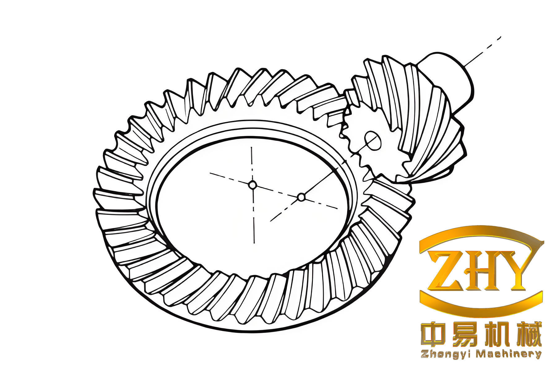
In the field of power transmission, the hypoid bevel gear stands out for its superior performance characteristics. The unique offset between the axes of the pinion and the gear allows for higher torque transmission, smoother operation, and reduced noise compared to traditional bevel gears. These advantages have cemented its role as a critical component in demanding applications such as automotive rear axles, aerospace systems, and heavy industrial machinery. As performance requirements escalate, particularly with the advancement of electric and high-performance vehicles, the precise manufacturing and assembly of these gears become paramount. One of the most telling indicators of a properly manufactured and assembled hypoid bevel gear set is the contact pattern formed between the mating tooth surfaces during operation.
The contact pattern, or contact spot, is the visible area on the tooth flank where active contact and load transfer occur. Its size, location, shape, and orientation are direct reflections of the gear’s geometric accuracy, alignment, and potential for smooth, quiet, and durable operation. A poorly positioned or sized contact pattern can lead to premature wear, excessive noise, pitting, and ultimately, catastrophic gear failure. Traditionally, the inspection of this vital feature has been a subjective process, reliant on the skilled eye of an experienced technician using visual inspection, often aided by a coating of marking compound (e.g., Prussian blue) and a roll test. This method, while practical, suffers from significant drawbacks: low accuracy, poor repeatability, qualitative rather than quantitative results, and an inability to integrate into automated, high-volume production lines. The industry’s push towards Industry 4.0 and smart manufacturing has created a pressing need for an objective, automated, and real-time method to evaluate hypoid bevel gear contact patterns.
The convergence of high-resolution digital imaging, powerful computing hardware, and sophisticated image processing algorithms presents a compelling solution to this challenge. By treating the contact pattern inspection as a computer vision problem, it is possible to move from subjective human judgment to precise, quantitative mathematical evaluation. This article details a comprehensive image processing methodology designed specifically for the analysis of contact patterns on hypoid bevel gear teeth. The proposed workflow encompasses image acquisition, pre-processing, feature extraction, geometric parameterization of the complex tooth flank, and finally, the quantitative assessment of the contact pattern’s key attributes.
1. Methodology: A Step-by-Step Image Processing Pipeline
The core of the proposed system is a structured pipeline that transforms a raw image of a gear tooth into a set of quantitative metrics describing the contact pattern. The process can be divided into four major sequential stages: Image Acquisition & Pre-processing, Edge Detection & Feature Isolation, Tooth Flank Parameterization, and Contact Pattern Quantification.
1.1. Image Acquisition and Pre-processing
The first step involves capturing a high-quality digital image of the gear tooth with the visible contact pattern. This is typically achieved using a fixed-mount industrial CCD or CMOS camera equipped with appropriate lighting to ensure high contrast between the contact area (often stained with marking compound) and the bare metal of the hypoid bevel gear tooth. Consistent lighting and camera positioning are crucial for repeatable measurements.
The raw color image (commonly in RGB format) contains redundant information for edge detection purposes. Converting it to a grayscale image reduces computational complexity. The conversion is performed using a weighted average that accounts for the human eye’s sensitivity to different colors:
$$ Y = 0.299R + 0.587G + 0.114B $$
where \(Y\) is the resulting grayscale intensity, and \(R\), \(G\), and \(B\) are the red, green, and blue channel intensities, respectively. The weights 0.299, 0.587, and 0.114 are standard values derived from photometric science.
Industrial images are often contaminated with noise from various sources (sensor noise, electrical interference, etc.). To mitigate this, image smoothing is applied. A common and effective technique is the Gaussian filter, which convolves the image with a Gaussian kernel. The discrete 2D Gaussian kernel \(G\) of size \((2k+1)\times(2k+1)\) is given by:
$$ G(x, y) = \frac{1}{2\pi\sigma^2} e^{-\frac{x^2+y^2}{2\sigma^2}} $$
for \(x, y \in \{-k, -k+1, …, k-1, k\}\), where \(\sigma\) is the standard deviation controlling the degree of blur. The smoothed image \(I_{smooth}\) is obtained by:
$$ I_{smooth}(i, j) = \sum_{x=-k}^{k} \sum_{y=-k}^{k} I(i-x, j-y) \cdot G(x, y) $$
This step suppresses high-frequency noise while preserving the essential structural edges of the tooth and contact pattern.
1.2. Edge Detection and Feature Isolation
Edges in an image correspond to abrupt changes in intensity, marking the boundaries of objects—in this case, the boundary of the gear tooth and the boundary of the contact spot. Edge detection is the process of identifying these points. The Canny edge detector is widely regarded as an optimal method due to its good performance in terms of noise immunity and detection accuracy. It involves multiple steps:
- Gradient Calculation: Compute the intensity gradient using derivatives of a Gaussian filter. The gradients in the x and y directions, \(G_x\) and \(G_y\), are found using convolution with Sobel or similar kernels:
$$ G_x = \begin{bmatrix} -1 & 0 & +1 \\ -2 & 0 & +2 \\ -1 & 0 & +1 \end{bmatrix} * I_{smooth}, \quad G_y = \begin{bmatrix} -1 & -2 & -1 \\ 0 & 0 & 0 \\ +1 & +2 & +1 \end{bmatrix} * I_{smooth} $$
The gradient magnitude \(M\) and direction \(\theta\) are then:
$$ M = \sqrt{G_x^2 + G_y^2}, \quad \theta = \arctan2(G_y, G_x) $$ - Non-Maximum Suppression: Thin the edges by preserving only local maxima in the gradient direction.
- Double Thresholding and Hysteresis: Use two thresholds (\(T_{high}\) and \(T_{low}\)) to classify edge pixels. Strong pixels (gradient > \(T_{high}\)) are retained. Weak pixels (gradient between \(T_{low}\) and \(T_{high}\)) are kept only if they are connected to strong pixels.
The result is a binary image where white pixels represent detected edges. Subsequent morphological operations like opening and closing can be used to clean up small spurious edges and connect broken segments. Finally, based on geometric constraints (e.g., the expected polygonal shape of the tooth boundary), the algorithm isolates the closed contour representing the tooth flank and the closed contour(s) representing the contact spot.
| Edge Detection Operator | Key Principle | Advantages | Disadvantages for Gear Analysis |
|---|---|---|---|
| Sobel | Gradient approximation using simple convolution | Simple, fast computation | Poor noise immunity, thick edges |
| Prewitt | Similar to Sobel with different kernel | Simple implementation | Noise sensitive, not directional |
| Laplacian of Gaussian (LoG) | Detects edges via zero-crossings of second derivative | Good localization | Responds strongly to noise and isolated points |
| Canny | Multi-stage optimal detector with noise filtering | Low error rate, good localization, single response | Computationally more intensive, requires parameter tuning |
1.3. Tooth Flank Parameterization via Surface Grid Construction
The curved, non-developable surface of a hypoid bevel gear tooth presents a significant challenge. To quantitatively locate a contact spot, we need a coordinate system mapped onto the tooth flank itself. The proposed solution is to construct a parametric surface grid that digitally “covers” the tooth flank area as seen in the 2D image.
The four extracted boundary curves of the tooth (\(C_{top}\), \(C_{root}\), \(C_{heel}\), \(C_{toe}\)) are first approximated mathematically. Using a least-squares polynomial fit of degree 5 provides a good balance between accuracy and smoothness for each curve \(i\):
$$ y_i(x) = a_{5,i}x^5 + a_{4,i}x^4 + a_{3,i}x^3 + a_{2,i}x^2 + a_{1,i}x + a_{0,i} $$
The intersections of these fitted curves define the four corner points of the tooth flank region: \(P_{00}\) (heel-toe), \(P_{01}\) (heel-root), \(P_{10}\) (top-toe), \(P_{11}\) (top-root).
Each boundary curve is then re-parameterized by its arc length \(s\), which is a natural and smooth parameter. For a curve defined as \(r(t) = (x(t), y(t))\), the arc length from parameter \(t_0\) to \(t\) is:
$$ s(t) = \int_{t_0}^{t} \sqrt{ \left( \frac{dx}{dt} \right)^2 + \left( \frac{dy}{dt} \right)^2 } dt $$
In practice, for a discrete set of \(n+1\) points along the curve, the cumulative chord length is used to approximate \(s\). We then obtain functions \(x_i(s)\) and \(y_i(s)\) for each boundary \(i\) via interpolation or fitting.
To construct a surface over the quadrilateral region defined by the four boundaries, the Coons patch technique is employed. A linear Coons patch defines a surface \(S(u,v)\) that interpolates the four boundary curves, where \(u\) and \(v\) are normalized parameters in \([0,1]\). Let \(C_1(u)\) and \(C_3(u)\) be the opposing heel and toe boundaries, and \(C_2(v)\) and \(C_4(v)\) be the opposing top and root boundaries, all now parameterized by their normalized arc length. The Coons patch is given by the Boolean sum:
$$ S(u,v) = L_u(u,v) + L_v(u,v) – B(u,v) $$
where:
- \(L_u(u,v) = (1-v)C_1(u) + v C_3(u)\) is the linear interpolation between the heel and toe curves.
- \(L_v(u,v) = (1-u)C_2(v) + u C_4(v)\) is the linear interpolation between the top and root curves.
- \(B(u,v) = (1-u)(1-v)P_{00} + u(1-v)P_{10} + (1-u)v P_{01} + uv P_{11}\) is the bilinear interpolant of the four corners.
Thus, the final surface point in image coordinates \((X, Y)\) for any \((u,v)\) is:
$$ S(u,v) = \begin{bmatrix} X(u,v) \\ Y(u,v) \end{bmatrix} = \begin{bmatrix} (1-v)X_1(u) + v X_3(u) + (1-u)X_2(v) + u X_4(v) – B_x(u,v) \\ (1-v)Y_1(u) + v Y_3(u) + (1-u)Y_2(v) + u Y_4(v) – B_y(u,v) \end{bmatrix} $$
This construction creates a smooth mapping from the 2D parametric (u,v)-space (a unit square) to the distorted quadrilateral region of the hypoid bevel gear tooth flank in the image (x,y)-space. Every pixel within the tooth boundary corresponds to a unique \((u,v)\) coordinate pair.
1.4. Contact Pattern Quantification in Parametric Space
With the mapping \(S(u,v)\) established, every point \(p_i = (x_i, y_i)\) on the extracted contact spot boundary can be transformed into its corresponding parametric coordinate \((u_i, v_i)\). This is achieved by solving the inverse mapping problem: for a given \((x_i, y_i)\), find \((u_i, v_i)\) such that \(S(u_i, v_i) = (x_i, y_i)\). This typically requires a numerical root-finding approach like the Newton-Raphson method in two dimensions.
The collection of \((u_i, v_i)\) points now represents the contact pattern within the normalized parametric domain. This transformation is powerful because it “unfolds” or “normalizes” the curved tooth flank into a standard domain for analysis. The inherently curved and asymmetric shape of the physical tooth (with heel, toe, top, root) maps to the unit square in parametric space, where the boundaries are straight and axis-aligned: \(u=0\) (heel), \(u=1\) (toe), \(v=0\) (top), \(v=1\) (root).
To visually match the elongated shape of a typical hypoid bevel gear tooth, a simple affine scaling can be applied to the parametric coordinates for display purposes without affecting the quantitative metrics. For instance, scaling \(u\) by a factor of 5 and making \(v\) a linear function of \(u\) (e.g., \(v’ = v \cdot (0.2u + 1)\)) can transform the unit square into a trapezoidal shape reminiscent of the actual tooth.
Within this consistent parametric framework, key quantitative metrics of the contact pattern can be computed robustly:
- Centroid Location: The center of mass of the contact spot in (u,v)-space indicates its positional bias.
$$ u_c = \frac{1}{A}\iint_{\Omega} u \, d\Omega, \quad v_c = \frac{1}{A}\iint_{\Omega} v \, d\Omega $$
where \(\Omega\) is the region of the contact spot and \(A\) is its area in parametric space. - Area: The normalized area \(A\) of the contact pattern, computed via the shoelace formula on the polygon defined by \((u_i, v_i)\) points.
$$ A = \frac{1}{2} \left| \sum_{i=1}^{n} (u_i v_{i+1} – u_{i+1} v_i) \right| $$
where \(v_{n+1} = v_1\). - Orientation: The principal axis of the contact pattern can be found by performing Principal Component Analysis (PCA) on the set of \((u_i, v_i)\) points. The eigenvector corresponding to the largest eigenvalue defines the major axis direction \(\theta_p\) in the uv-plane.
$$ \Sigma = \begin{bmatrix} \text{Var}(u) & \text{Cov}(u,v) \\ \text{Cov}(u,v) & \text{Var}(v) \end{bmatrix}, \quad \Sigma \mathbf{v} = \lambda \mathbf{v} $$ - Dimensions: The length \(L\) (along the major axis) and width \(W\) (along the minor axis) can be derived from the extreme projections of the boundary points onto these axes.
- Distance to Boundaries: Critical clearances, such as the minimum distance from the contact pattern centroid to the heel (\(u_c\)), toe (\(1-u_c\)), top (\(v_c\)), and root (\(1-v_c\)) edges, are trivially calculated in parametric space.
| Evaluation Metric | Mathematical Definition in (u,v)-Space | Engineering Significance |
|---|---|---|
| Centroid (u_c, v_c) | $$ u_c = \frac{\sum u_i}{N}, v_c = \frac{\sum v_i}{N} $$ | Indicates pattern shift towards heel/toe or top/root; crucial for diagnosing misalignment. |
| Normalized Area (A) | $$ A = \iint_{\Omega} du\, dv $$ | Measures load distribution potential. Too small indicates high stress; too large risks edge contact. |
| Orientation Angle (θ) | Angle of major axis from u-axis via PCA. | Should align with the local surface curvature. Abnormal rotation indicates lead or spiral angle errors. |
| Aspect Ratio (AR) | $$ AR = L_{major} / L_{minor} $$ | Describes shape elongation. Related to the conformity of the mating surfaces. |
| Edge Clearance (C) | $$ C_{heel} = u_{min}, C_{toe} = 1 – u_{max}, etc. $$ | Absolute minimum distance from pattern to any flank boundary. Prevents stress concentration at edges. |
2. Experimental Validation and Discussion
The proposed methodology was implemented and tested using a software environment capable of image processing and numerical computation, such as MATLAB or Python with OpenCV and SciPy libraries. A dataset of images from various hypoid bevel gear sets, with contact patterns generated under different assembly conditions (e.g., pinion offset, mounting distance variations), was processed.
The edge detection stage confirmed the superiority of the Canny detector for this application. While simpler operators like Sobel were faster, they produced noisier, thicker boundaries that complicated the subsequent contour isolation. The Canny detector, with appropriately tuned thresholds, yielded clean, single-pixel wide contours essential for accurate boundary fitting.
The core of the method, the Coons patch parameterization, proved robust. By using arc-length parameterization for the boundaries, the resulting (u,v) coordinate lines were evenly spaced along the edges, providing a smooth and intuitive grid over the tooth flank. The inverse mapping from image coordinates to (u,v) coordinates was computationally the most intensive step but was reliably solved using iterative methods, ensuring every contact spot pixel was accurately mapped.
The true value of the method was demonstrated in the quantification phase. For example, a gear set with a known, deliberately introduced pinion offset error produced a contact pattern whose centroid in the (u,v)-space showed a clear and measurable shift towards the heel edge (low \(u_c\) value) and possibly the root (high \(v_c\) value). This shift could be quantified to within a fraction of a percent of the normalized tooth length, providing a precise diagnostic measure. Similarly, a pattern that was too small yielded a low normalized area \(A\), while one that was over-extended and risked edge contact showed critically low edge clearance values \(C_{toe}\) or \(C_{heel}\).
The parametric representation also allows for the establishment of clear, numerical acceptance criteria. Instead of relying on vague descriptions like “pattern centered,” tolerances can be set on the metrics: e.g., \(0.45 < u_c < 0.55\), \(0.40 < v_c < 0.60\), \(A > 0.15\), \(C_{min} > 0.05\). This enables fully automated Go/No-Go decisions in a production line setting.
| Test Case | Induced Error | Observed Centroid Shift (u_c, v_c) | Change in Area (A) | Diagnosis from Parametric Metrics |
|---|---|---|---|---|
| Reference (Good) | None | (0.50, 0.48) | 0.22 | Centered, adequate area. |
| Case 1 | Increased Pinion Offset | (0.35, 0.52) | 0.18 | Significant shift toward heel (low u_c). |
| Case 2 | Decreased Mounting Distance | (0.51, 0.65) | 0.15 | Shift toward root (high v_c), area reduced. |
| Case 3 | Axial Misalignment | (0.49, 0.47) | 0.10 | Area severely reduced, indicating loss of contact. |
3. Conclusion and Future Perspectives
This article has presented a comprehensive and novel image processing framework for the quantitative evaluation of contact patterns on hypoid bevel gear teeth. The method transitions the critical quality control process from a subjective, skill-dependent visual inspection to an objective, automated, and mathematically rigorous analysis. By integrating advanced edge detection, geometric curve fitting, and surface parameterization via Coons patches, the complex curved flank of the gear is mapped to a normalized parametric domain. This mapping facilitates the precise calculation of definitive metrics—centroid location, area, orientation, and edge clearances—that directly correlate with the gear’s meshing quality and assembly correctness.
The implications for manufacturing are significant. This system can be deployed as a core component of an automated in-line or end-of-line inspection station for hypoid bevel gear assemblies. Coupled with a robotic handling system and a fixed vision setup, it can provide 100% inspection coverage with consistent, documented results, feeding statistical process control (SPC) systems and enabling traceability. It reduces reliance on highly specialized labor and eliminates human variability from the inspection process.
Future work can extend this methodology in several promising directions. Firstly, integrating 3D stereo vision or structured light scanning could allow the method to account for the actual three-dimensional topography of the tooth flank, moving beyond the 2D projection assumption. This would be particularly valuable for analyzing very large gears or patterns with significant depth variation. Secondly, machine learning algorithms, particularly deep convolutional neural networks (CNNs), could be trained on large datasets of processed images to not only measure the pattern but also to directly classify the type of assembly error (e.g., “excessive offset,” “incorrect backlash”) from the raw or pre-processed image, potentially speeding up diagnosis. Finally, the quantitative metrics generated can be fed back in a closed-loop system to adaptive machining centers or assembly robots, enabling real-time correction of the manufacturing process to ensure every hypoid bevel gear set meets its stringent design specifications. The fusion of computer vision, computational geometry, and advanced manufacturing embodied in this method represents a substantial step towards the intelligent, data-driven production of high-performance power transmission components.