
The strain wave gear, also commonly referred to as a harmonic drive, represents a pivotal advancement in precision gearing technology. Its operation relies on the controlled elastic deformation of a flexible component to achieve motion transmission, offering unparalleled advantages in compactness, high reduction ratios, zero-backlash operation, and coaxial shaft design. These attributes make it indispensable in fields demanding high precision and reliability, such as aerospace robotics, satellite positioning systems, and advanced medical equipment. At the heart of this system lies the flexspline—a thin-walled, cup-shaped gear that undergoes cyclical elastic deformation during operation. This very mechanism that grants the strain wave gear its unique benefits also subjects the flexspline to complex, time-varying stress states, making fatigue life a critical design constraint. Consequently, accurately predicting the stress distribution within the flexspline, particularly at stress concentration points like the tooth root fillet, is paramount for optimizing performance, ensuring reliability, and extending service life.
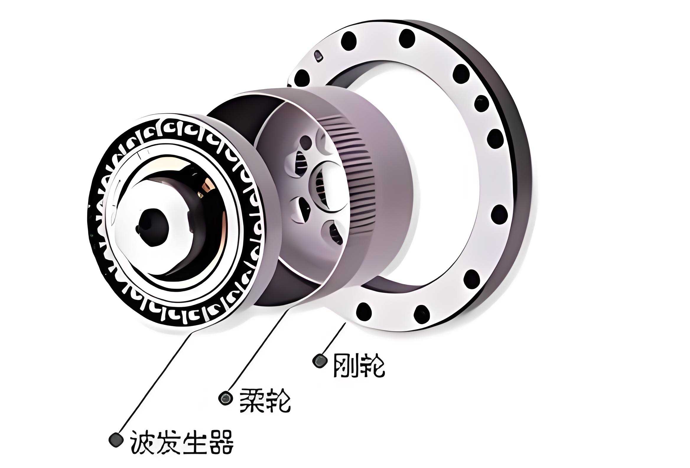
The core operational principle of a cup-type strain wave gear involves three primary components: a rigid Circular Spline (CS), a flexible Flexspline (FS), and an elliptical Wave Generator (WG). The wave generator, often incorporating a cam and a specially designed “Flex Bearing,” is inserted into the bore of the flexspline. This forces the flexspline to adopt an elliptical shape. The flexspline typically has two fewer teeth than the circular spline. At the major axis of the ellipse, the teeth of the flexspline fully engage with the teeth of the circular spline. At the minor axis, they are completely disengaged. As the wave generator rotates, the points of engagement move circumferentially, causing a slow relative rotation between the flexspline and the circular spline. This process subjects the flexspline to a fully-reversed, cyclical stress field, with maximum stresses typically occurring in the cup diaphragm and at the root of the teeth near the major axis positions.
Experimental measurement of these stresses is notoriously challenging due to the small size, complex geometry, and moving contact interfaces within a sealed strain wave gear assembly. Strain gauges can be applied, but their placement is limited, they may interfere with the gear mesh, and capturing the complete spatial and temporal stress field is impractical. This is where advanced numerical modeling becomes an essential tool. This article details a sophisticated three-dimensional Finite Element Method (FEM) approach for modeling the complete strain wave gear system, with a focus on accurately capturing the stress state in the flexspline.
1. Comprehensive 3D Numerical Modeling Methodology
Creating a predictive model of a strain wave gear requires carefully addressing multiple, simultaneous nonlinearities: large deformations of the flexspline, complex contact between multiple bodies (wave generator bearing, flexspline, circular spline), and material nonlinearity if considered. A simplistic model treating the wave generator as a rigid ellipse and ignoring detailed contact physics will yield inaccurate stress results. The methodology presented here employs a multi-faceted strategy to realistically simulate the system’s mechanics.
1.1 Modeling of the Wave Generator and Flex Bearing
The wave generator assembly is the source of deformation in the strain wave gear. Modeling every ball in the flex bearing with explicit contact against the races is computationally prohibitive for system-level stress analysis. An effective and efficient simplification is the “Spring Analogy” method. In this approach, the force-displacement relationship between the bearing races at each ball location is modeled using a nonlinear spring element. The stiffness of this spring is derived from Hertzian contact theory, which calculates the local deformation between two elastic curved bodies under load.
The force in the spring is governed by:
$$F = -k(d – \Delta)$$
where \(F\) is the contact force, \(k\) is the contact stiffness (dependent on the load and material properties), \(d\) is the relative displacement between the inner and outer race connection points, and \(\Delta\) is the initial radial clearance of the bearing. For a given torque load, the number of bearing balls in load-sharing zones can be estimated from static equilibrium. The contact stiffness for these balls is then calculated based on the approximated load per ball and held constant, as studies have shown the variation in load per ball across the contact arc is relatively small for system-level stress analysis purposes. This method captures the essential load-transfer mechanism of the bearing without the extreme computational cost of explicit ball modeling.
1.2 Modeling of the Lubricant Film Interface
Between the outer race of the flex bearing and the inner surface of the flexspline, a thin film of lubricant is present. While primarily for reducing wear, this film has a small but non-negligible compliance that can affect the pressure distribution on the flexspline’s inner wall. To model this, a layer of specialized interface elements is inserted. These elements are active only when the surfaces are in contact (i.e., when the gap is zero or negative). They possess orthotropic material properties, being very compliant in the tangential direction to allow shear but having a defined stiffness in the normal direction to transmit pressure from the bearing to the flexspline.
The material constants for this thin film layer, defined in a cylindrical coordinate system aligned with the flexspline, are typically approximated as:
$$
\begin{bmatrix}
\sigma_{rr} \\
\sigma_{\theta\theta} \\
\tau_{r\theta}
\end{bmatrix}
=
\begin{bmatrix}
E_{rr} & 0 & 0 \\
0 & E_{\theta\theta} & 0 \\
0 & 0 & G_{r\theta}
\end{bmatrix}
\begin{bmatrix}
\epsilon_{rr} \\
\epsilon_{\theta\theta} \\
\gamma_{r\theta}
\end{bmatrix}
$$
where \(E_{rr} \approx 3.09 \text{ MPa}\) is the radial elastic modulus (modeling the film’s squeeze stiffness), \(E_{\theta\theta} \approx 2.06 \text{ MPa}\) is the circumferential modulus, and \(G_{r\theta} = E_{\theta\theta}\) is the shear modulus. This approach provides a more realistic pressure boundary condition on the flexspline compared to a perfectly rigid contact assumption.
1.3 Modeling Flexspline-Circular Spline Tooth Contact
The most critical interaction for stress analysis is the meshing between the flexspline and circular spline teeth. This is a dynamic, moving contact problem with changing engagement conditions. To handle this efficiently in a static or quasi-static analysis, a “Gap Element” or “Contact Element” strategy is employed. Potential contact points on the tooth flanks are identified, and pairs of nodes (one on the FS, one on the CS) are connected by a uniaxial spring element aligned normal to the contact surface. This element has the following logic:
- If the gap between the nodes is open (\(gap > 0\)), the element contributes zero stiffness (no force).
- If the gap is closed (\(gap \leq 0\)), the element activates with a very high stiffness (\(E \approx 206 \text{ GPa}\)), simulating metal-to-metal contact and preventing penetration.
The force in this element, \(F_c\), is calculated as \(F_c = k_c \cdot \text{max}(0, -gap)\), where \(k_c\) is the contact stiffness. The sum of these forces across all tooth pairs gives the total mesh load. Since the circular spline is much stiffer than the flexspline, it is often modeled as a rigid body to reduce computational complexity, which is a standard and valid assumption for stress analysis focused on the flexspline. The figure below conceptually illustrates the insertion of these contact elements at different mesh depths.
| Component | Simplified Modeling Method | Key Parameters / Equations | Purpose / Advantage |
|---|---|---|---|
| Wave Generator Bearing | Nonlinear Spring Analogy | $$F = -k(d – \Delta)$$, Hertzian stiffness \(k\) | Efficiently captures load transfer without modeling each ball explicitly. |
| Lubricant Film | Orthotropic Interface Layer | $$E_{rr} \approx 3.09 \text{ MPa}, E_{\theta\theta} \approx 2.06 \text{ MPa}$$ | Provides realistic compliant pressure boundary on flexspline inner wall. |
| Gear Tooth Contact | Gap / Contact Elements | $$F_c = k_c \cdot \text{max}(0, -gap)$$ | Efficiently models moving contact and prevents penetration in static analysis. |
| Circular Spline | Rigid Body Assumption | Constraint all DOFs | Significantly reduces model size and solve time; valid due to high stiffness. |
2. Analysis of Flexspline Deformation and Stress Results
Implementing the above modeling strategy in a commercial finite element analysis (FEA) software package allows for a detailed investigation of the strain wave gear assembly under load. The model is typically solved in several steps: first applying the wave generator ellipse deformation (pre-stress), then applying the output torque load to the flexspline, and finally, incrementally rotating the wave generator to simulate different positions in the engagement cycle.
2.1 Deformation and Constraint Effect
A primary finding from the numerical model is the critical constraint effect imposed by the circular spline on the flexspline’s free deformation. If the model is run with only the wave generator deforming the flexspline and without activating the tooth contact elements, the flexspline deforms freely into a more pronounced elliptical shape. However, when the contact elements are active, the meshing teeth of the circular spline physically constrain this deformation. The resulting loaded shape shows a smaller radial displacement at the major axis compared to the free-deformation case. This constrained deformation state is the physically correct one and aligns closely with experimental observations using optical or coordinate measurement techniques. It conclusively demonstrates that system-level modeling, rather than analyzing the flexspline in isolation, is necessary for accuracy.
2.2 Circumferential Stress Distribution
The most valuable output of the analysis is the detailed stress field within the flexspline. Under a significant output torque (e.g., 329 N·m), the model reveals a classic and critical stress pattern. High tensile stresses develop on one side of the major axis in the cup diaphragm and tooth root regions, while high compressive stresses develop on the opposite side. As the wave generator rotates, a specific material point on the flexspline will cyclically experience this full reversal from tension to compression. This fully-reversed cyclic loading is the primary driver of fatigue failure in strain wave gear flexsplines.
The maximum stress magnitudes are consistently found in two critical zones: 1) the inner fillet radius of the cup diaphragm where it meets the cylindrical tooth band, and 2) the root fillet of the teeth engaged near the major axis of the wave generator. The stress concentration in these fillet regions is significantly influenced by the geometry (fillet radius, wall thickness profile) and the applied torque.
The circumferential (hoop) stress at the tooth root is of particular interest for gear strength assessment. The numerical model allows us to plot this stress around the entire circumference of the flexspline. The plot reveals a characteristic bimodal distribution with two peaks located symmetrically on either side of the major axis (around ±110° from the minor axis). This pattern occurs because the maximum mesh force and bending moment on the tooth occur not exactly at the major axis, but at points where the leverage and engagement conditions are most severe.
| Stress Feature | Location | Cause / Mechanism | Implication for Design |
|---|---|---|---|
| Maximum Tensile Stress | Diaphragm inner fillet & tooth root on one side of major axis. | Combined bending from elliptical deformation and tensile hoop stress from torque transmission. | Primary site for fatigue crack initiation. Critical for S-N curve and life calculation. |
| Maximum Compressive Stress | Diaphragm inner fillet & tooth root on opposite side of major axis. | Combined bending from elliptical deformation and compressive hoop stress. | Although compression is less damaging in fatigue, it completes the fully-reversed cycle. |
| Bimodal Hoop Stress Distribution | Tooth root circumference, peaks at ~±110° from minor axis. | Complex interaction of tooth bending, shear, and circumferential membrane stresses. | Validates model against experimental strain gauge data; identifies critical engagement zones. |
| Stress Concentration | All fillet radii (diaphragm, tooth root). | Geometric discontinuity causing local stress increase. | Optimization of fillet radii and transition profiles is crucial for life extension. |
3. Model Validation and Parametric Studies
3.1 Quantitative Validation Against Experimental Data
The true test of any numerical model is its correlation with empirical data. When the circumferential stress at the tooth root predicted by the detailed FEA model is superimposed on experimental measurements obtained from carefully placed strain gauges, the correlation is striking. Both the qualitative shape (the bimodal distribution with two peaks) and the quantitative magnitude of the stress are accurately captured. For instance, under a specific load, experiments may show a peak stress of approximately 450 MPa, while the FEA model predicts a peak around 400-420 MPa. The slight discrepancy can be attributed to uncertainties in material properties, exact boundary conditions, and measurement accuracy, but the agreement is well within acceptable engineering margins for a complex system like a strain wave gear. This validation provides high confidence in the model’s predictive capability.
3.2 Parametric Analysis and Virtual Testing
One of the greatest strengths of a validated numerical model is the ability to conduct virtual parametric studies that would be prohibitively expensive or time-consuming physically. The model enables the systematic investigation of how key design variables influence the critical stress state in the strain wave gear flexspline.
- Torque Load: The model confirms that stress magnitudes in the flexspline scale nearly linearly with applied output torque. It can predict stress states at the operational torque limit, a condition extremely difficult to instrument and measure reliably in physical tests without risk of failure.
- Wave Generator Ellipticity (Cam Profile): The amount of radial deformation imposed by the wave generator is a primary design parameter. The model can quantify the trade-off: increased ellipticity allows for more teeth in simultaneous engagement (higher torque capacity) but also increases the bending stress in the flexspline diaphragm and teeth, potentially reducing fatigue life.
- Flexspline Geometry: Parameters such as cup diaphragm thickness, tooth band thickness, fillet radii at the diaphragm and tooth root, and the overall profile can be varied parametrically. The FEA model can directly compute the resulting change in maximum stress, enabling shape optimization to minimize stress concentration. For example, optimizing the diaphragm profile from a constant thickness to a contoured one (thicker near the shaft connection, thinner near the tooth band) can significantly reduce peak stress.
- Tooth Geometry: The influence of pressure angle, addendum/dedendum modification, and tooth profile (involute vs. S-shaped) on the load distribution and root stress can be studied in detail, guiding the selection for optimal strength and smooth meshing in the strain wave gear.
The sensitivity of the maximum principal stress (\(\sigma_{max}\)) to key parameters can often be expressed through derived empirical relationships from multiple FEA runs. A generalized form might look like:
$$
\sigma_{max} \approx C_T \cdot T + C_{\delta} \cdot \delta + \sigma_0
$$
where \(C_T\) is the sensitivity coefficient to torque \(T\), \(C_{\delta}\) is the sensitivity coefficient to wave generator deflection \(\delta\), and \(\sigma_0\) is the pre-stress from assembly. The coefficients are determined from the parametric study data.
4. Implications for Fatigue Life Prediction and Design Optimization
The accurate stress results from this advanced numerical modeling feed directly into the most important engineering task: predicting the fatigue life of the strain wave gear flexspline and optimizing its design.
4.1 From Stress to Fatigue Life
With the full-field, time-varying stress tensor available from the FEA model for a complete rotation cycle, engineers can apply multiaxial fatigue criteria (such as the Dang Van, Crossland, or Findley criterion) to calculate an equivalent alternating stress and mean stress at every point in the model. This is far superior to using nominal stresses. Combining this with the material’s S-N (Stress-Number of cycles) curve, often adjusted for surface finish, size, and reliability factors using Marin’s equation, allows for a local strain-life or stress-life approach to fatigue analysis.
$$
N_f = f(\sigma_{alt}, \sigma_{mean}, \text{material properties})
$$
The model identifies the critical point with the shortest predicted life (usually in the diaphragm or tooth root fillet), providing a quantitative life estimate for a given load spectrum. This enables reliable design for a specified service life or the calculation of a safe operating torque for a required life.
4.2 Design Optimization Workflow
The integrated modeling approach enables a structured optimization workflow for the strain wave gear:
- Baseline Analysis: Model the initial design to establish stress benchmarks and identify critical zones.
- Parameterization: Define key geometric variables (e.g., diaphragm thickness profile \(t(r)\), fillet radii \(R_{fillet}\), tooth geometry parameters).
- Design of Experiments (DOE): Use the FEA model as a solver to run a set of analyses across the defined parameter space.
- Response Surface & Optimization: Fit a meta-model (response surface) to the FEA results. Use an optimization algorithm (e.g., gradient-based, genetic algorithm) to find the parameter set that minimizes maximum stress or maximizes fatigue life while respecting constraints like weight, stiffness, and manufacturability.
- Verification: Run a final, detailed FEA on the optimized design to verify performance improvements.
This process, powered by the accurate numerical model described, allows designers to push the performance boundaries of strain wave gear systems—achieving higher torque density, longer life, and greater reliability—which are constant demands in advanced robotics and aerospace applications.
5. Conclusion
The accurate assessment of stress within the flexspline is the cornerstone of reliable strain wave gear design. This article has detailed a robust and validated three-dimensional finite element modeling methodology that moves beyond simplifications to capture the essential physics of the system. By employing a spring analogy for the wave generator bearing, specialized elements for the lubricant film interface, and active contact elements for the tooth mesh, the model efficiently yet accurately simulates the complex, constrained deformation of the flexspline under load. The results provide detailed insight into the critical circumferential stress distribution, revealing the characteristic bimodal pattern and identifying the diaphragm and tooth root fillets as primary fatigue risk zones.
Quantitative validation against experimental strain gauge data confirms the model’s predictive accuracy. This validated model unlocks powerful capabilities for the engineer: it serves as a virtual test bench for conducting parametric studies, evaluating the impact of geometric changes, and predicting fatigue life with high confidence. Ultimately, this advanced numerical modeling approach is not merely an analytical tool but an enabling technology for the optimization and innovation of next-generation strain wave gear systems, ensuring they meet the ever-increasing demands for precision, compactness, and durability in high-tech industries.