
The reliable operation of propulsion systems is paramount in marine engineering. Among these, the combined diesel and gas turbine (CODAG) systems frequently employ complex helical gear transmissions due to their high load capacity and smooth engagement characteristics. These helical gear sets operate under severe and dynamic conditions characterized by heavy loads, high speeds, and potential shock impacts. In such a demanding environment, gear tooth failure, particularly tooth breakage, is a critical and prevalent fault mode. A broken tooth drastically alters the contact conditions between mating gears, modifying the internal dynamic excitation within the transmission system. The time-varying meshing stiffness (TVMS) is a fundamental parameter governing the dynamic behavior of a gear pair, serving as a primary source of parametric excitation. Consequently, investigating the evolution of TVMS under tooth breakage faults is not merely an academic exercise but an essential step for developing effective condition monitoring and prognostic strategies for marine gearboxes, ultimately enhancing operational safety and reliability.
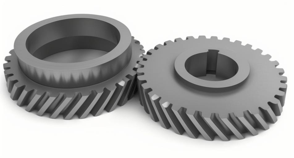
While extensive research exists on gear faults like cracks, spalling, and pitting, the specific case of tooth breakage in helical gears requires a more nuanced approach. Existing studies often simplify the breakage geometry, typically assuming fractures either parallel to the face width or parallel to the line of contact, with predefined breakage angles and extents. However, in reality, an overload-induced fracture can occur at any arbitrary angle relative to the gear axis. Calculations based on oversimplified breakage models can lead to significant deviations from the actual meshing stiffness, limiting the accuracy of subsequent dynamic response analyses and fault diagnosis algorithms. Therefore, this article aims to develop a generalized analytical methodology for calculating the meshing stiffness of a helical gear pair subjected to tooth breakage at any arbitrary angle. The core of this methodology lies in accurately modeling the effective length of contact lines, which is directly proportional to the mesh stiffness, under various broken tooth geometries.
Classification of Tooth Breakage Modes in Helical Gears
Overload breakage, often initiating at the tooth tip where bending stress is highest, can manifest in different geometric forms depending on the fracture propagation path. To systematically analyze their impact, we categorize tooth breakage into two distinct modes based on the orientation of the fracture surface relative to the instantaneous line of contact between mating helical gear teeth.
Mode I: Breakage Parallel to the Line of Contact. In this mode, the fracture surface is assumed to be parallel to the direction of the contact line on the tooth flank. This represents a special case where the breakage angle θ, defined as the angle between the fracture edge and the gear axis, is 90°. The damaged region is characterized by a loss of material along a segment of the tooth, with the breakage extent defined by a length parameter \(l_a\), measured along the tooth profile.
Mode II: Breakage Not Parallel to the Line of Contact. This is the general case where the fracture surface is oriented at an arbitrary angle θ (where θ ≠ 90°) relative to the gear axis. The geometry of the missing tooth fragment is now defined by both the fixed breakage initiation point (e.g., at the tip) and the breakage angle θ. The extent of damage is characterized by a different length parameter \(l_b\), which is a function of θ and the position of the breakage point.
| Breakage Mode | Description | Key Geometric Parameter | Schematic Representation |
|---|---|---|---|
| Mode I | Fracture surface parallel to the contact line. | Breakage length \(l_a\) (θ = 90°). | Rectangular missing region aligned with contact path. |
| Mode II | Fracture surface at an arbitrary angle θ to the gear axis. | Breakage angle θ and initiation point, defining length \(l_b\). | Trapezoidal or triangular missing region. |
Mathematical Modeling of Contact Line Length for Helical Gears
The time-varying contact line length is the foundation for calculating the meshing stiffness of a helical gear pair. For a healthy gear, the contact lines move across the plane of action as the gears rotate.
Contact Line Model for a Healthy Helical Gear Pair
We establish a coordinate system on the plane of action. The x-axis is perpendicular to the contact lines, and the y-axis is parallel to them. The displacement along the x-axis over time is given by the rolling motion:
$$x(t) = v \cos(\beta_b) t$$
where \(v\) is the velocity along the line of action and \(\beta_b\) is the base circle helix angle.
The total contact line length at any time \(t\) can be visualized as the difference between the time-varying positions of the leading edge \(l_1(t)\) and the trailing edge \(l_2(t)\) of the contact zone on the tooth flank. These position functions are piecewise linear, governed by the gear geometry and kinematics. For a standard helical gear with axial contact ratio \(\varepsilon_{\beta}\) and transverse contact ratio \(\varepsilon_{\alpha}\), the functions over one mesh cycle \(T_c\) (the time to pass one base pitch \(p_{bt}\)) are:
Leading edge function:
$$
l_1(t) =
\begin{cases}
\frac{v t \cos\beta_b}{\tan\beta_b} + L_{CD}\sin\beta_b, & 0 \leq t \leq \varepsilon_{\beta} T_c \\
(-v t + L_{CD})\sin\beta_b + \frac{v \varepsilon_{\beta} T_c}{\sin\beta_b}, & \varepsilon_{\beta} T_c \leq t \leq \varepsilon_{\gamma} T_c
\end{cases}
$$
Trailing edge function:
$$
l_2(t) =
\begin{cases}
-v t \sin\beta_b + L_{CD}\sin\beta_b, & 0 \leq t \leq \varepsilon_{\alpha} T_c \\
\frac{v t \cos\beta_b}{\tan\beta_b} + L_{CD}\sin\beta_b, & \varepsilon_{\alpha} T_c \leq t \leq \varepsilon_{\gamma} T_c
\end{cases}
$$
Here, \(\varepsilon_{\gamma} = \varepsilon_{\alpha} + \varepsilon_{\beta}\) is the total contact ratio, and \(L_{CD}\) is a constant related to the initial engagement position. The time-varying contact line length for a single tooth pair is:
$$L(t) = l_1(t) – l_2(t)$$
Contact Line Model with Tooth Breakage (Mode I: θ = 90°)
When a tooth is broken parallel to the contact line (Mode I), a rectangular region of the tooth flank is missing. During the meshing period when the contact line would normally pass through this region, the effective contact length is zero. The contact only resumes when the remaining healthy part of the tooth enters the mesh. Let \(t_1\) be the time when the trailing edge of the contact zone reaches the end of the broken segment (point F). The modified contact line function \(L'(t)\) becomes:
$$
L'(t) =
\begin{cases}
0, & t \in [0, t_1] \\
l_1(t) – l_2(t), & t \in [t_1, \varepsilon_{\gamma} T_c]
\end{cases}
$$
The time \(t_1\) is directly proportional to the breakage length \(l_a\).
Contact Line Model with Tooth Breakage (Mode II: θ ≠ 90°)
For the general breakage mode, the fracture line at angle θ will intersect the moving contact zone boundaries \(l_1(t)\) and \(l_2(t)\) at two different instants, \(t_2\) and \(t_3\). The fracture line itself can be described by a time-dependent function \(l_{E’F’}(t)\) based on its slope (\(\tan\theta\)) and its intersection point with \(l_2(t)\) at \(t_2\):
$$l_{E’F’}(t) = v t \cos\beta_b \tan\theta + l_2(t_2) – \frac{1}{4}v \varepsilon_{\gamma} T_c \cos\beta_b \tan\theta, \quad t \in [\min(t_2, t_3), \max(t_2, t_3)]$$
The modification to the leading and trailing edge functions depends on whether θ is less than or greater than 90°.
Case 1: θ < 90°. The breakage region is ahead of the fixed fracture point E’. Contact is lost from the start of mesh until the trailing edge \(l_2(t)\) reaches E’ at \(t_2\). From \(t_2\) to \(t_3\), the contact line is partially formed along the fracture edge \(l_{E’F’}(t)\). After \(t_3\), the contact resumes normally on the intact part of the tooth.
$$
l_1′(t) =
\begin{cases}
0, & t \in [0, t_2] \\
l_{E’F’}(t), & t \in [t_2, t_3] \\
l_1(t), & t \in [t_3, \varepsilon_{\gamma} T_c]
\end{cases}
\quad \text{and} \quad
l_2′(t) =
\begin{cases}
0, & t \in [0, t_2] \\
l_2(t), & t \in [t_2, \varepsilon_{\gamma} T_c]
\end{cases}
$$
Case 2: θ > 90°. The breakage region is behind the fixed fracture point E’. Contact is lost from the start of mesh until the leading edge \(l_1(t)\) reaches F’ at \(t_3\). From \(t_3\) to \(t_2\), the contact line is partially formed. After \(t_2\), contact resumes normally.
$$
l_1′(t) =
\begin{cases}
0, & t \in [0, t_3] \\
l_1(t), & t \in [t_3, \varepsilon_{\gamma} T_c]
\end{cases}
\quad \text{and} \quad
l_2′(t) =
\begin{cases}
0, & t \in [0, t_3] \\
l_{E’F’}(t), & t \in [t_3, t_2] \\
l_2(t), & t \in [t_2, \varepsilon_{\gamma} T_c]
\end{cases}
$$
The effective contact line length for the faulty tooth pair is then calculated as:
$$L'(t) = l_1′(t) – l_2′(t)$$
This generalized formulation allows for the calculation of the contact line for any breakage angle θ, providing a crucial input for stiffness calculation.
Calculation of Time-Varying Meshing Stiffness
In a helical gear pair, multiple tooth pairs are in contact simultaneously. The total effective contact line length at any time \(t\) is the sum of the individual contact line lengths \(L’_i(t)\) for all \(M\) engaged tooth pairs:
$$L_{total}(t) = \sum_{i=1}^{M} L’_i(t)$$
According to the ISO standard and fundamental contact mechanics, the mesh stiffness of a gear pair is directly proportional to the total length of contact lines, assuming a uniform stiffness per unit length \(k_0\) along the contact line. Therefore, the time-varying meshing stiffness \(k_m(t)\) is given by:
$$k_m(t) = k_0 \cdot L_{total}(t)$$
The constant \(k_0\) can be derived from the ISO 6336 standard formulas for calculating the mesh stiffness of a single tooth pair per unit face width, incorporating bending, shear, axial compressive, and contact (Hertzian) deformations. For a helical gear, this is typically the stiffness in the normal plane.
Stiffness Characteristics Under Mode I Breakage (θ = 90°)
Analyzing a marine helical gear pair with parameters: \(z_1/z_2 = 18/71\), \(b = 50\) mm, \(m_n = 3\) mm, \(\alpha = 20°\), \(\beta = 13°\), we calculate the single-tooth-pair and total mesh stiffness for different breakage lengths \(l_a\).
| Breakage Length \(l_a\) | Single-Tooth Stiffness in Fault Zone | Total Mesh Stiffness Impact | Recovery Behavior |
|---|---|---|---|
| 0 (Healthy) | Normal parabolic profile. | Normal, multi-step profile. | N/A |
| \(l_a = \frac{1}{3}l_m\) | Zero for a duration \(\Delta t_1\). | Reduced by ~1/3 of one tooth’s contribution for \(\Delta t_1\). | Instantaneous recovery after \(\Delta t_1\). |
| \(l_a = \frac{2}{3}l_m\) | Zero for a longer duration \(\Delta t_2 > \Delta t_1\). | Reduced by a greater amount for \(\Delta t_2\). | Instantaneous recovery after \(\Delta t_2\). |
| \(l_a = l_m\) (Full segment) | Zero for the entire single-tooth mesh period. | One tooth pair contributes zero stiffness for its full engagement. | Instantaneous recovery when next pair engages. |
The key observation is that for Mode I breakage, the stiffness loss is total within the broken segment and the transition from faulty to healthy contact is abrupt, leading to a sharp, step-like recovery in the total mesh stiffness signal. The duration and depth of the stiffness reduction are directly proportional to \(l_a\).
Stiffness Characteristics Under Mode II Breakage (θ ≠ 90°)
For the general case, we fix the breakage initiation point and analyze for two angles: \(\theta = 90° – \beta_b\) and \(\theta = 90° + \beta_b\).
| Breakage Angle θ | Stiffness in Fault Zone | Transition Region Behavior | Physical Interpretation |
|---|---|---|---|
| \(\theta < 90°\) (e.g., \(90° – \beta_b\)) | Single-tooth stiffness is zero initially, then partial. | Gradual, linear increase in single-tooth stiffness from zero to full as contact area recovers. | The slanted fracture causes the contact line to be re-established gradually across the face width. |
| \(\theta > 90°\) (e.g., \(90° + \beta_b\)) | Single-tooth stiffness is zero initially, then partial. | Gradual, linear increase in single-tooth stiffness from zero to full as contact area recovers. | The slanted fracture causes a different pattern of gradual recovery. |
The defining characteristic of Mode II breakage is the gradual recovery of stiffness. Unlike the instantaneous jump in Mode I, here the single-tooth-pair stiffness ramps up linearly from zero to its nominal value as the meshing progresses from the broken region into the healthy part of the tooth. This results in a distinctive, trapezoidal-shaped depression in the total mesh stiffness curve, rather than a rectangular pulse. The slope of the recovery ramp is a function of the breakage angle θ.
Discussion and Implications for Condition Monitoring
The developed methodology provides a direct link between the physical geometry of a broken tooth in a helical gear and its resulting meshing stiffness function. The differences in stiffness signatures between Mode I and Mode II breakage have significant implications for vibration-based fault diagnosis.
The sharp, impulse-like stiffness change from a Mode I breakage is likely to excite higher-frequency resonant modes of the gearbox structure, producing transient impulses in the vibration signal synchronous with the gear’s rotation. In the frequency domain, this may lead to increased sidebands around the gear mesh frequency and its harmonics.
Conversely, the gradual stiffness change from a Mode II breakage acts as a slower modulation of the mesh stiffness. This may produce a stronger amplitude modulation effect on the vibration signal at the gear’s rotational frequency. The distinct shape of the stiffness modulation (trapezoidal vs. rectangular) could potentially be inverted from carefully analyzed vibration or transmission error measurements, offering a pathway to not only detect a breakage but also estimate its geometric parameters (angle θ and extent \(l_b\)).
Furthermore, the reduction in mesh stiffness leads to an increase in the loaded static transmission error, which is the primary kinematic excitation in gear dynamics. This altered excitation pattern will change the system’s dynamic response, potentially increasing vibration levels and dynamic loads on other components. Accurate modeling of this faulty stiffness is therefore critical for predicting the overall dynamic behavior and assessing the risk of secondary damage in a marine transmission system.
Conclusion
This analysis presents a generalized framework for calculating the time-varying meshing stiffness of a helical gear pair with a tooth breakage fault. By classifying breakage into two modes—parallel (Mode I) and non-parallel (Mode II) to the contact line—and deriving the corresponding time-varying contact line length formulas for any breakage angle θ, we enable a more accurate representation of real-world fault geometries. The stiffness is then computed based on the fundamental proportionality between total contact line length and mesh stiffness.
The key findings are:
- For Mode I Breakage (θ = 90°): The stiffness of the affected tooth pair drops to zero completely for a duration proportional to the breakage length \(l_a\). The total mesh stiffness exhibits a rectangular reduction pulse. Recovery to normal stiffness is instantaneous once the meshing moves past the broken segment.
- For Mode II Breakage (θ ≠ 90°): The stiffness loss is also total initially, but the recovery is gradual and linear as the contact line progressively sweeps across the slanted fracture surface. This results in a trapezoidal reduction pulse in the total mesh stiffness profile. The slope of recovery is indicative of the breakage angle.
This work moves beyond simplified breakage models, providing a tool for generating accurate faulted stiffness profiles. These profiles are essential inputs for high-fidelity dynamic simulations of marine helical gear transmissions, which in turn are crucial for developing advanced, model-based fault detection and prognosis systems aimed at ensuring the reliability and safety of marine propulsion systems operating under severe conditions.