
In precision motion control systems, such as those found in aerospace servo actuators, the transmission mechanism plays a critical role in determining positional accuracy, dynamic response, and load capacity. The planetary roller screw assembly has emerged as a superior alternative to the conventional ball screw due to its higher load-carrying capacity, greater stiffness, and longer operational life. This electromechanical device efficiently converts rotational motion into precise linear displacement. Its operation relies on multi-point contact through complex spatial thread surfaces between the screw, the rollers, and the nut. However, this very contact mechanism introduces nonlinear stiffness behavior. Under significant axial loads, the resulting elastic deformations within the assembly generate positional errors that can critically impact the performance of high-precision systems. Therefore, developing an accurate analytical model for the axial stiffness of a planetary roller screw assembly is fundamental for dynamic system modeling, performance prediction, and optimal design. This article establishes a comprehensive stiffness model based on differential geometry and Hertzian contact theory, analyzes the influence of key design parameters, and validates the model through experimental testing.
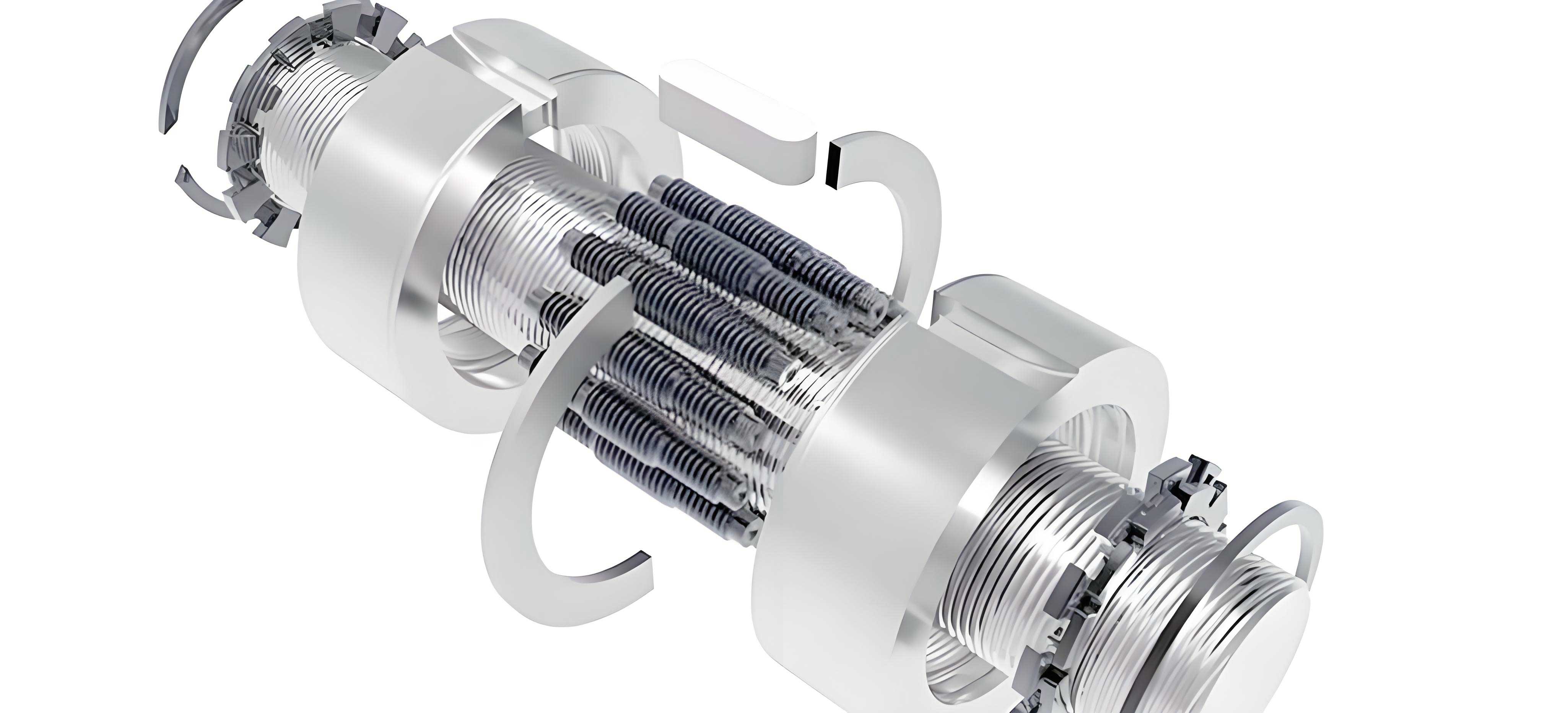
The fundamental structure of a planetary roller screw assembly comprises four primary components: a central screw, a surrounding nut, multiple cylindrical rollers distributed circumferentially, and a retainer or planetary guide that maintains the roller arrangement. Both the screw and the rollers feature external threads, while the nut contains an internal thread. The rollers are engaged between the screw and nut threads. When the screw is rotated, typically by a motor, the rollers are driven. They consequently rotate about their own axes, revolve around the screw axis (planetate), and translate axially. This compound motion drives the nut along the screw’s axis, producing linear output. The kinematic relationship between the nut’s axial displacement \( s \) and the screw’s rotation angle \( \theta_S \) is governed by the thread leads and the geometry of the contacting parts. For a standard design where the roller thread lead equals the nut thread lead, the relationship can be expressed as:
$$ s = \frac{P_{eff} \cdot \theta_S}{2\pi} $$
where \( P_{eff} \) is the effective lead of the assembly. A more detailed geometric derivation considering the screw lead \( P_S \) and roller lead \( P_R \) yields:
$$ s = \frac{\theta_S (r_R P_S + r_S P_R)}{2\pi r_R} \cdot \frac{r_S + 2r_R}{2r_S + 2r_R} $$
Here, \( r_S \) and \( r_R \) represent the pitch radii of the screw and roller threads, respectively. This kinematic foundation is essential for understanding load paths and subsequent deformations.
The overall axial stiffness of a planetary roller screw assembly is a series combination of the stiffnesses of its constituent elements under load. Conceptually, the load path from the nut to the fixed end of the screw involves several elastic components in series. For a load applied to the nut, the sequence of deformations includes: compression/extension of the nut’s cylindrical body, bending and shear of the nut’s thread teeth, Hertzian contact deformation at the nut-roller interface, compression/extension and thread tooth deflection of the roller, Hertzian contact deformation at the roller-screw interface, bending and shear of the screw’s thread teeth, and finally, compression/extension of the screw’s cylindrical body. Therefore, the total axial compliance \( 1/K_{total} \) is the sum of the compliances of each of these elements.
$$ \frac{1}{K_{total}} = \frac{1}{K_{body,N}} + \frac{1}{K_{thread,N}} + \frac{1}{K_{contact,NR}} + \frac{1}{K_{body,R}} + \frac{1}{K_{thread,R}} + \frac{1}{K_{contact,RS}} + \frac{1}{K_{thread,S}} + \frac{1}{K_{body,S}} $$
Modeling each component accurately is key to predicting the system’s stiffness.
Component Stiffness Modeling
1. Body Stiffness of Screw, Nut, and Rollers
The screw, nut, and roller bodies can be modeled as solid or hollow cylinders under axial tension/compression. Their stiffness values are typically orders of magnitude higher than the thread contact stiffnesses but are included for completeness. Assuming a linear elastic material with Young’s modulus \( E \) and a cross-sectional area \( A \), the axial stiffness over an effective length \( L_{eff} \) (often related to the pitch) is:
$$ K_{body} = \frac{E \cdot A}{L_{eff}} $$
For the rollers, which are numerous, the combined stiffness of all rollers in parallel must be considered. If there are \( n_R \) rollers, the effective body stiffness contribution from the rollers is \( n_R \cdot K_{body,R} \).
2. Thread Contact Stiffness Based on Hertzian Theory
The most critical and complex aspect of modeling a planetary roller screw assembly’s stiffness is characterizing the contact stiffness at the thread interfaces. Unlike ball screws with point contacts, the planetary roller screw assembly involves line contacts between conjugate helical surfaces. The contact is treated as a series of discrete points along the thread flank. The key step is determining the principal curvatures of the contacting thread surfaces at the point of load application.
The thread profile of a planetary roller screw assembly is often a modified triangular form. The roller thread can be approximated as having an arc profile. Using differential geometry, the surface of a thread can be described parametrically. For the upper flank of a roller thread, a point on the surface can be located by parameters \( a \) (radial distance from roller axis) and \( \theta \) (angular position):
$$ \mathbf{r_R}(a, \theta) = \begin{bmatrix} a \cos\theta \\ a \sin\theta \\ \frac{L}{2\pi}\theta + \sqrt{r_p^2 – a^2} – \sqrt{r_p^2 – r_R^2} + p \end{bmatrix} $$
where \( L \) is the thread lead, \( p \) is a phase constant, \( r_R \) is the roller root radius, and \( r_p \) is the radius of the thread profile arc, related to the contact angle \( \beta \) by \( r_p = r_R / \sin \beta \). The unit normal vector \( \mathbf{N_R} \) at a point on this surface is crucial for contact analysis.
From the parametric equations, the first and second fundamental forms of the surface are computed. The coefficients of the first fundamental form (\( E, F, G \)) and the second fundamental form (\( L, M, N \)) are derived from partial derivatives of \( \mathbf{r} \) and \( \mathbf{N} \). For the screw thread upper surface, these coefficients take forms like:
$$ E_{ST} = 1 + \tan^2\beta_S, \quad F_{ST} = -\frac{L_S \tan\beta_S}{2\pi}, \quad G_{ST} = a^2 + \left(\frac{L_S}{2\pi}\right)^2 $$
$$ L_{ST} = 0, \quad M_{ST} = -\cos\beta_S \sin\alpha_S, \quad N_{ST} = -a \sin\beta_S $$
where \( \alpha_S \) is the helix angle. The Gaussian curvature \( K_G \) and mean curvature \( H \) are then found from:
$$ K_G = \frac{LN – M^2}{EG – F^2}, \quad H = \frac{EN + GL – 2FM}{2(EG – F^2)} $$
The principal curvatures \( \kappa_1 \) and \( \kappa_2 \) are the roots of \( \kappa^2 – 2H\kappa + K_G = 0 \):
$$ \kappa_{1,2} = H \pm \sqrt{H^2 – K_G} $$
Their reciprocals give the principal radii of curvature: \( R_1 = 1/\kappa_1, R_2 = 1/\kappa_2 \). This process is repeated for both contacting bodies (e.g., screw and roller) at the presumed contact point.
With the four principal radii (\( R_{1I}, R_{2I} \) for body I and \( R_{1II}, R_{2II} \) for body II), the geometry of contact is defined. The composite curvatures \( \Theta \) and \( \chi \) are calculated:
$$ \Theta + \chi = \frac{1}{2}\left( \frac{1}{R_{1I}} + \frac{1}{R_{2I}} + \frac{1}{R_{1II}} + \frac{1}{R_{2II}} \right) $$
$$ \Theta – \chi = \frac{1}{2}\left[ \left( \frac{1}{R_{1I}} – \frac{1}{R_{2I}} \right)^2 + \left( \frac{1}{R_{1II}} – \frac{1}{R_{2II}} \right)^2 + 2\left( \frac{1}{R_{1I}} – \frac{1}{R_{2I}} \right)\left( \frac{1}{R_{1II}} – \frac{1}{R_{2II}} \right)\cos 2\gamma \right]^{1/2} $$
where \( \gamma \) is the angle between the principal curvature axes of the two surfaces. The equivalent radius \( R_e \) is then:
$$ R_e = \left( \frac{\Theta}{\chi} \right)^{-1/2} $$
According to Hertzian contact theory for elastic bodies, the normal approach \( \delta \) (contact deformation) under a load \( Q \) is given by:
$$ \delta_H = \mathcal{F}^2 \left( \frac{9 Q^2}{16 {E^*}^2 R_e} \right)^{1/3} $$
where \( \mathcal{F} \) is a dimensionless factor dependent on the curvature ratio, and \( E^* \) is the equivalent elastic modulus:
$$ \frac{1}{E^*} = \frac{1 – \nu_I^2}{E_I} + \frac{1 – \nu_{II}^2}{E_{II}} $$
with \( E \) and \( \nu \) being the Young’s modulus and Poisson’s ratio of the respective materials. The axial component of this deformation, which contributes to the overall axial compliance of the planetary roller screw assembly, is \( \delta_{H,axial} = \delta_H / (\cos\beta \cos\alpha) \), where \( \beta \) is the thread contact angle and \( \alpha \) is the helix angle. The contact stiffness for a single thread pair is thus \( K_{contact} = Q / \delta_{H,axial} \).
3. Thread Tooth Bending Stiffness
Each thread tooth can be idealized as a short, radially oriented cantilever beam or an annular plate segment fixed at the root and loaded at the pitch diameter. A more accurate model treats the thread helix as a thin annular plate under a concentrated radial load \( \omega \) at radius \( r_0 \). The axial deflection \( \delta_{TB} \) at the load point can be derived using plate theory and is of the form:
$$ \delta_{TB} = -\frac{\omega a}{C_8} \left( \frac{r_0 C_9}{b} – L_9 \right) \frac{r_2}{D} F_2 + \frac{\omega r_0}{b} \frac{r_3}{D} F_3 – \omega \frac{r_3}{D} G_3 $$
where \( a, b \) are outer and inner radii of the annular section, \( t \) is tooth thickness, and \( C_8, C_9, L_9, D, F_2, F_3, G_3 \) are constants or functions derived from the boundary conditions and geometry of the annular plate model. The thread tooth stiffness is then \( K_{thread} = \omega / \delta_{TB} \). This stiffness must be calculated for both the nut and screw threads, and for the roller threads which are loaded on both flanks.
4. Synthesis of Overall Axial Stiffness
The load is shared among several engaged thread pairs along the nut. A load distribution factor \( \xi_i \) describes the fraction of the total axial load \( F_a \) carried by the \( i \)-th engaged thread pair: \( Q_i = \xi_i F_a \). The factors \( \xi_i \) are not uniform due to elastic interactions; they are determined by solving a system of deformation compatibility equations. For the \( i \)-th and \( (i+1) \)-th threads on a roller and nut, the compatibility condition enforces that the difference in approach between adjacent teeth must equal the stretching of the column of material between them:
$$ \frac{Q_{i-1} – Q_i}{K_{i}^{RN}} – \frac{Q_i – Q_{i+1}}{K_{i+1}^{RN}} = Q_i \left( \frac{1}{K_{i}^{NB}} + \frac{1}{K_{i}^{RB}} \right) $$
where \( K_{i}^{RN} = \left( \frac{1}{K_{thread,R,i}} + \frac{1}{K_{thread,N,i}} + \frac{1}{K_{contact,NR,i}} \right)^{-1} \) is the combined stiffness of the roller thread, nut thread, and their contact at position \( i \). \( K^{NB} \) and \( K^{RB} \) are the axial column stiffnesses of the nut and roller body sections between threads. Solving this system for all engaged threads yields the load distribution \( \xi_i \).
The total axial deformation \( \Delta_{loaded} \) of the engaged zone is the sum of deformations from all components under this distributed load. The stiffness of the loaded zone \( K_{loaded} \) is \( F_a / \Delta_{loaded} \). Finally, the stiffness \( K_{unloaded} \) of the screw shaft section beyond the nut (if present) acts in series with the loaded zone stiffness. This section is a simple cylinder:
$$ K_{unloaded} = \frac{E_S \pi r_s^2}{L_{unloaded}} $$
where \( r_s \) is the screw root radius and \( L_{unloaded} \) is its length. The total axial stiffness of the planetary roller screw assembly is therefore:
$$ \frac{1}{K_{total}} = \frac{1}{K_{loaded}} + \frac{1}{K_{unloaded}} $$
Parametric Analysis and Simulation
Using the developed model, the influence of key design and operational parameters on the axial stiffness of a planetary roller screw assembly can be systematically analyzed. The following table summarizes the base parameters for a representative assembly used in simulation.
| Parameter | Symbol | Value |
|---|---|---|
| Nut Thread Diameter | \( D_N \) | 35 mm |
| Screw Thread Diameter | \( D_S \) | 21 mm |
| Roller Diameter | \( D_R \) | 7 mm |
| Number of Thread Starts (Screw/Nut) | \( n \) | 5 |
| Screw Lead Angle | \( \alpha_S \) | 1.74° |
| Roller/Nut Lead Angle | \( \alpha_R \) | 1.04° |
| Contact Angle (Baseline) | \( \beta \) | 45° |
| Number of Rollers (Baseline) | \( n_R \) | 10 |
| Young’s Modulus (All Steel Parts) | \( E \) | 210 GPa |
| Poisson’s Ratio | \( \nu \) | 0.3 |
1. Load Distribution and Its Effect
The model reveals a non-uniform load distribution across the engaged threads. The load factor \( \xi_i \) typically peaks at the first few load-bearing threads near the point of load application and decreases rapidly for subsequent threads. This concentration becomes more severe under higher total loads. A uniform distribution is ideal for maximizing capacity and life. The design should aim to have a sufficient number of engaged threads such that the maximum load factor \( \xi_{max} \) remains below a safe limit relative to the material’s yield strength. This analysis is critical for ensuring the reliability of the planetary roller screw assembly under high loads.
2. Influence of Thread Contact Angle (\( \beta \))
The thread contact angle significantly affects both the load-carrying geometry and the Hertzian contact conditions. Simulations show that increasing \( \beta \) leads to a substantial increase in axial stiffness. A larger contact angle improves the normal force component for a given axial load, reducing contact stresses and deformations. However, an excessively large angle may compromise other performance aspects like back-driving resistance or manufacturability. An angle of 45° is often a practical optimum, balancing high stiffness with other functional requirements of the planetary roller screw assembly.
3. Influence of Number of Rollers (\( n_R \))
The number of rollers is a primary design lever for scaling the capacity and stiffness of the assembly. Since the rollers share the total load in parallel, increasing \( n_R \) directly and significantly increases the overall axial stiffness. The relationship is roughly linear for the contact and thread tooth deflections. However, increasing the roller count also increases the complexity, mass, and friction within the system. There exists a trade-off, and the optimal number depends on the specific application requirements for stiffness, size, weight, and efficiency of the planetary roller screw assembly.
4. Effect of Clearance and Eccentricity
Manufacturing tolerances lead to clearances in the thread mesh and potential eccentricities in roller positioning. The model can account for a radial offset or “eccentricity” \( e \) of a roller’s axis relative to its nominal position. This misalignment alters the local contact geometry and preload, leading to an uneven load distribution among the rollers. Rollers with larger effective negative clearance (tighter fit) will carry disproportionately higher loads, reducing the overall stiffness compared to a perfectly aligned assembly. Similarly, axial clearance in the thread engagement reduces the number of simultaneously load-bearing threads under light loads, degrading initial stiffness. The presented stiffness model, by incorporating detailed geometry, can quantify these detrimental effects, guiding tolerance specification for the planetary roller screw assembly.
The table below summarizes simulated stiffness values for varying loads and parameters, illustrating the nonlinear stiffening behavior and parametric influences.
| Axial Load (N) | Baseline Stiffness (N/μm) | Stiffness with \( \beta = 50^\circ \) (N/μm) | Stiffness with \( n_R = 12 \) (N/μm) |
|---|---|---|---|
| 10,000 | 52.1 | 58.7 (+12.7%) | 62.5 (+20.0%) |
| 30,000 | 68.3 | 78.9 (+15.5%) | 82.0 (+20.1%) |
| 50,000 | 78.5 | 92.1 (+17.3%) | 94.8 (+20.8%) |
| 70,000 | 86.0 | 102.5 (+19.2%) | 105.3 (+22.4%) |
Experimental Validation
To validate the analytical stiffness model for the planetary roller screw assembly, a dedicated static stiffness test rig was designed and constructed. The core principle is to apply a precisely measured axial force to the assembly and measure the resulting elastic axial displacement.
Test Setup: The planetary roller screw assembly is mounted vertically between two rigid support plates. The screw is prevented from rotating using an anti-rotation key/link. A calibrated hydraulic or mechanical loading mechanism applies a compressive axial force to the nut (or screw), which is measured by a high-precision load cell. The relative axial displacement between the nut and a reference point on the screw (or housing) is measured using non-contact displacement sensors, such as eddy-current probes with sub-micrometer resolution. The setup must isolate the deformation of the test specimen from the compliance of the fixture. The stiffness of the support structure (\( >5\times10^9 \, N/m \)) was designed to be at least an order of magnitude higher than the expected stiffness of the planetary roller screw assembly (\( \sim 2\times10^8 \, N/m \)), ensuring its contribution is negligible.
Procedure: The axial load is applied in incremental steps from zero to the maximum rated load and then unloaded. At each step, the steady-state force and displacement readings are recorded. The axial stiffness at a given load is calculated as the incremental change in force divided by the incremental change in displacement (\( K = \Delta F / \Delta \delta \)). The process is repeated to ensure repeatability.
Results and Comparison: The experimental load-displacement curve exhibits the characteristic nonlinear stiffening, with compliance being highest at low loads and decreasing as load increases. The measured stiffness values across the load range are compared with those predicted by the analytical model. The comparison for a specific test specimen is shown in the conceptual data below. The model predictions show good agreement with experimental measurements across the operational load range. The maximum observed error is approximately 8.3%. The slight over-prediction of stiffness by the model is expected and can be attributed to factors not fully captured in the ideal model, such as: minor misalignments in the test fixture contributing to measured displacement, the influence of unmodeled thread root fillets, and possible slight variations in material properties or surface finish from the ideal assumptions.
Conclusion
This article has presented a comprehensive methodology for analyzing the axial stiffness of a planetary roller screw assembly. The model integrates the stiffness contributions of the component bodies, the thread teeth in bending, and, most importantly, the nonlinear Hertzian contact at the threaded interfaces. The use of differential geometry to accurately characterize the principal curvatures of the complex thread surfaces represents a significant advancement over simplified models, leading to a more physically accurate prediction of stiffness.
The parametric analysis demonstrates that the axial stiffness of a planetary roller screw assembly increases nonlinearly with applied load and is strongly enhanced by a larger thread contact angle and a greater number of rollers. However, design trade-offs must be considered. Manufacturing imperfections like clearance and eccentricity can lead to uneven load sharing, reducing overall stiffness and necessitating careful tolerance control.
Experimental validation confirms the accuracy of the proposed analytical model, with errors within an acceptable engineering margin. This validated model serves as a powerful tool for designers to predict the performance of a planetary roller screw assembly, optimize its parameters for specific applications requiring high stiffness and precision, and integrate it effectively into higher-level system dynamic models. The insights gained facilitate the development of more reliable and accurate servo systems for demanding fields such as aerospace and robotics.