
In modern engineering applications, gear drives are ubiquitous across industries such as aerospace, marine, automotive, machine tools, and construction machinery. Among these, the helical gear stands out due to its superior load distribution, smoother operation, and higher torque capacity compared to spur gears. However, gear systems are prone to failures, with statistics indicating that approximately 80% of faults in transmission machinery and 10% in rotating machinery are gear-related. Common failure modes include tooth pitting and tooth breakage, which are directly linked to contact and bending stresses during meshing. Therefore, it is crucial to analyze the meshing characteristics of helical gear pairs to ensure durability and reliability. In this study, we employ a node generation technique within ANSYS APDL to develop a precise finite element model for helical gears, enabling a detailed investigation into stress and strain distributions during meshing and the impact of design parameters like root fillet radius.
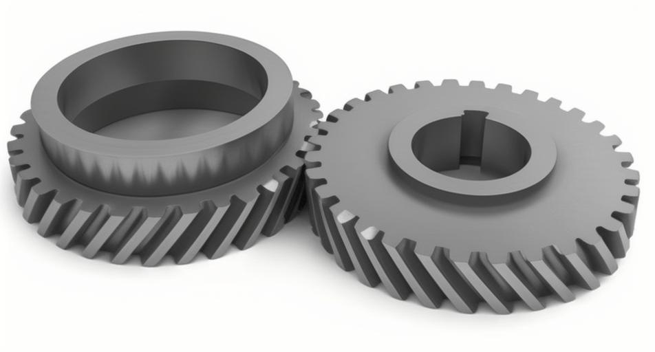
The meshing of helical gears involves highly nonlinear contact problems with complex boundary conditions, making accurate modeling challenging. Traditional methods, such as analytical approaches or simplified numerical simulations, often fail to capture real-world operating conditions. While CAD software like Pro/Engineer or UG can be used for modeling and importing into analysis tools like ANSYS or MSC.MARC, discrepancies due to precision and rounding errors during import can introduce inaccuracies. To overcome this, we utilize the ANSYS Parametric Design Language (APDL) with node generation technology to directly create a parameterized finite element model. This approach eliminates import-related errors and allows for controlled, high-quality meshing suitable for advanced contact analysis. Our methodology focuses on generating nodes based on the geometric principles of helical gears, ensuring precision and adaptability for various design scenarios.
Node generation begins with the fundamental parameters of a helical gear. The tooth profile in the transverse plane consists of an involute curve, root transition curve, root arc, and tip arc. We start by deriving the involute equations based on the gear’s basic geometry. For a helical gear, the transverse module \(m_t\) is related to the normal module \(m_n\) and helix angle \(\beta\) as:
$$m_t = \frac{m_n}{\cos(\beta)}$$
The base circle radius \(r_b\) for the transverse plane is calculated from the transverse pressure angle \(\alpha_t\) and pitch circle radius \(r_p\):
$$r_b = r_p \cos(\alpha_t)$$
where \(\alpha_t\) is derived from the normal pressure angle \(\alpha_n\) using:
$$\tan(\alpha_t) = \frac{\tan(\alpha_n)}{\cos(\beta)}$$
The involute curve in parametric form is given by:
$$x = r_b (\cos(\theta) + \theta \sin(\theta))$$
$$y = r_b (\sin(\theta) – \theta \cos(\theta))$$
where \(\theta\) is the roll angle. For the root and tip arcs, we define radii based on design standards, typically as multiples of the module. The root fillet radius \(R_a\) is often expressed as a factor \(\lambda\) of the transverse module:
$$R_a = \lambda m_t$$
where \(\lambda\) ranges from 0.15 to 0.50. We discretize these curves into nodes by sampling points along their lengths. For example, the involute segment is divided into \(n\) nodes with coordinates computed for each \(\theta_i\). The root and tip arcs are similarly discretized using circular equations. This process creates a set of nodes for one side of the tooth profile in the transverse plane.
Next, we mirror these nodes across the tooth centerline to form the complete transverse tooth profile. The nodes are then arranged in a sequence to define the contour. To extend this into a three-dimensional helical gear, we incorporate the helix. The helix lead \(L_h\) is calculated from the gear width \(b\) and helix angle \(\beta\):
$$L_h = \frac{2\pi r_p}{\tan(\beta)}$$
The axial coordinate \(z\) for each node is determined by projecting the transverse profile along the helix path. For a node with transverse coordinates \((x, y)\) and angular position \(\phi\) around the gear axis, the axial displacement is:
$$z = \frac{\phi}{\tan(\beta)}$$
We generate nodes at multiple cross-sections along the gear width, ensuring a smooth helical surface. These nodes are connected using SOLID185 elements, an 8-node brick element with three degrees of freedom per node (x, y, z), suitable for linear and nonlinear structural analysis. The node generation process bypasses traditional meshing steps, allowing for parametric control over mesh density and quality. Table 1 summarizes the key geometric parameters used in our helical gear model.
| Parameter | Symbol | Value |
|---|---|---|
| Normal module | \(m_n\) | 6 mm |
| Transverse module | \(m_t\) | 6.12 mm |
| Number of teeth (pinion) | \(z_1\) | 49 |
| Number of teeth (gear) | \(z_2\) | 64 |
| Helix angle | \(\beta\) | 11.6° |
| Normal pressure angle | \(\alpha_n\) | 20° |
| Transverse pressure angle | \(\alpha_t\) | 20.4° |
| Face width | \(b\) | 10 mm |
| Root fillet factor | \(\lambda\) | 0.38 (default) |
For meshing analysis, we create a gear pair consisting of a pinion (driving helical gear) and a gear (driven helical gear). The center distance \(a\) is computed from the pitch circle radii:
$$a = r_{p1} + r_{p2} = \frac{m_t (z_1 + z_2)}{2}$$
We establish local coordinate systems for both gears and position them at the calculated center distance. To simulate the meshing process, we rotate the gears through ten equally spaced positions over one engagement cycle. The total rotation angle \(\theta_{\text{total}}\) for a pair of teeth from start to end of engagement depends on the total contact ratio \(\varepsilon_{\gamma}\). For helical gears, the total contact ratio is the sum of the transverse contact ratio \(\varepsilon_{\alpha}\) and the axial contact ratio \(\varepsilon_{\beta}\):
$$\varepsilon_{\gamma} = \varepsilon_{\alpha} + \varepsilon_{\beta}$$
The transverse contact ratio is given by:
$$\varepsilon_{\alpha} = \frac{\sqrt{r_{a1}^2 – r_{b1}^2} + \sqrt{r_{a2}^2 – r_{b2}^2} – a \sin(\alpha_t)}{\pi m_t \cos(\alpha_t)}$$
where \(r_a\) is the tip radius and \(r_b\) is the base radius. The axial contact ratio is:
$$\varepsilon_{\beta} = \frac{b \tan(\beta)}{\pi m_t}$$
Thus, the rotation angle per tooth pair is:
$$\theta_{\text{total}} = \varepsilon_{\gamma} \times \frac{360^\circ}{z}$$
We divide \(\theta_{\text{total}}\) into ten increments to define the meshing positions. For each position, we adjust the angular orientation of the gears in their local coordinate systems to align the contacting teeth. Contact analysis is performed using surface-to-surface contact elements. The pinion and gear teeth surfaces are defined as contact pairs with a friction coefficient of 0.1. Boundary conditions are applied: the gear is constrained at its inner rim with all degrees of freedom fixed, while the pinion is constrained radially and axially but allowed to rotate. A torque \(T = 1000 \, \text{N·m}\) is applied to the pinion to simulate driving conditions. Material properties are set as steel with Young’s modulus \(E = 2.06 \times 10^5 \, \text{MPa}\) and Poisson’s ratio \(\nu = 0.3\).
The finite element analysis yields stress and strain distributions for each meshing position. We extract von Mises stress and equivalent elastic strain from the nodes on the tooth surfaces and roots. To quantify the meshing behavior, we compute average stress and strain values for the contacting nodes of the first contact pair across all ten positions. Additionally, we determine the percentage of total stress carried by each tooth in the contact pair relative to all contacting teeth. This allows us to assess load sharing and engagement dynamics. Table 2 presents the computed stress and strain values for the pinion and gear at key meshing positions.
| Meshing Position | Pinion Avg. Stress (MPa) | Gear Avg. Stress (MPa) | Pinion Avg. Strain (μm) | Gear Avg. Strain (μm) | Pinion Stress Share (%) | Gear Stress Share (%) |
|---|---|---|---|---|---|---|
| 1 (Start) | 45.2 | 52.1 | 22.5 | 5.3 | 18.7 | 31.2 |
| 2 | 58.7 | 65.4 | 18.9 | 7.1 | 24.3 | 39.8 |
| 4 | 68.3 | 72.8 | 16.2 | 8.5 | 28.5 | 48.0 |
| 6 | 73.5 | 71.9 | 16.8 | 8.2 | 50.9 | 46.5 |
| 8 | 69.8 | 66.7 | 15.4 | 7.6 | 38.2 | 35.4 |
| 10 (End) | 48.9 | 44.3 | 14.1 | 4.9 | 25.6 | 22.1 |
The results indicate that during meshing, the pinion tooth experiences increasing average stress in the initial phase, peaks around the mid-engagement position (e.g., position 6 at 73.5 MPa), and then decreases toward the end. The gear tooth shows a rapid stress rise at the start due to impact, stabilizes at a high level, and gradually declines. Strain patterns follow similar trends, with the pinion exhibiting higher deformation overall. The stress share analysis reveals that each tooth carries up to approximately 50% of the total contact stress during peak engagement, demonstrating effective load distribution in helical gears. This behavior aligns with the smooth and continuous engagement characteristic of helical gear systems, which reduces noise and vibration compared to spur gears.
To further investigate design influences, we analyze the effect of root fillet radius on meshing characteristics. The root fillet radius is varied by changing the factor \(\lambda\) from 0.15 to 0.50, while keeping other geometric parameters constant. For each value, we repeat the finite element analysis at the peak meshing position (position 6) and extract average and maximum stress and strain values at the tooth root and surface nodes. The root fillet radius directly impacts bending stress, as a larger radius reduces stress concentration. The bending stress \(\sigma_b\) at the root can be approximated using the Lewis formula modified for helical gears:
$$\sigma_b = \frac{F_t}{b m_n Y} K_v K_o K_m$$
where \(F_t\) is the tangential force, \(Y\) is the Lewis form factor, and \(K_v\), \(K_o\), \(K_m\) are velocity, overload, and mounting factors, respectively. However, our finite element analysis provides more detailed insights. Table 3 summarizes the results for different root fillet radii.
| Root Fillet Factor \(\lambda\) | Root Fillet Radius \(R_a\) (mm) | Pinion Root Avg. Stress (MPa) | Gear Root Avg. Stress (MPa) | Pinion Root Max Stress (MPa) | Gear Root Max Stress (MPa) | Surface Avg. Stress (MPa) | Surface Avg. Strain (μm) |
|---|---|---|---|---|---|---|---|
| 0.15 | 0.918 | 124.6 | 118.5 | 186.9 | 173.6 | 72.8 | 16.5 |
| 0.25 | 1.530 | 112.3 | 107.2 | 168.4 | 156.3 | 73.1 | 16.7 |
| 0.38 | 2.326 | 100.0 | 94.96 | 150.0 | 140.1 | 73.5 | 16.8 |
| 0.50 | 3.060 | 95.4 | 90.42 | 143.1 | 133.0 | 73.9 | 17.1 |
The data shows that as the root fillet radius increases, both average and maximum root stresses decrease significantly. For the pinion, average root stress drops from 124.6 MPa at \(\lambda = 0.15\) to 95.4 MPa at \(\lambda = 0.50\), a reduction of 29.2 MPa. Maximum root stress decreases by 43.8 MPa. Similar trends are observed for the gear. In contrast, surface contact stress and strain remain relatively unaffected, with fluctuations less than 1.2 MPa and 0.6 μm, respectively. This confirms that the root fillet radius primarily influences bending strength rather than contact conditions. The reduction in bending stress with larger radii enhances tooth resistance to breakage, a critical factor in helical gear design for high-load applications.
Our analysis also considers the dynamic aspects of helical gear meshing. The engagement stiffness varies during rotation due to changing contact lines. The mesh stiffness \(k_m\) for a helical gear pair can be expressed as a function of the contact ratio and tooth geometry:
$$k_m = \frac{1}{\frac{1}{k_{b1}} + \frac{1}{k_{b2}} + \frac{1}{k_{s1}} + \frac{1}{k_{s2}} + \frac{1}{k_h}}$$
where \(k_b\) is bending stiffness, \(k_s\) is shear stiffness, and \(k_h\) is Hertzian contact stiffness. For helical gears, the axial component adds complexity, but our finite element model captures these variations implicitly. We observe that the helical gear’s continuous engagement leads to smoother stiffness transitions, reducing vibration excitations. This contributes to the overall reliability of helical gear systems in precision machinery.
In summary, the node generation technique in ANSYS APDL provides a robust framework for modeling and analyzing helical gears. Our study demonstrates that helical gear meshing involves gradual stress buildup and decline, with peak stresses occurring mid-engagement and effective load sharing among teeth. The helical gear design ensures that no single tooth bears excessive load, with stress shares around 50% during critical phases. Parameter analysis reveals that increasing the root fillet radius substantially reduces bending stress without significantly affecting contact stress, offering a practical design lever for enhancing durability. These insights underscore the importance of detailed finite element analysis in optimizing helical gear performance. Future work could extend this approach to include thermal effects, lubrication, and dynamic loading for even more comprehensive helical gear design guidelines.
To further elaborate on the modeling process, the node generation algorithm involves iterative calculations for node coordinates. For instance, the involute segment is discretized using an angular step \(\Delta\theta\). The coordinates for each node \(i\) are:
$$x_i = r_b (\cos(\theta_i) + \theta_i \sin(\theta_i))$$
$$y_i = r_b (\sin(\theta_i) – \theta_i \cos(\theta_i))$$
$$\theta_i = \theta_{\text{start}} + i \Delta\theta$$
where \(\theta_{\text{start}}\) and \(\theta_{\text{end}}\) define the involute portion. For the helix, the axial position is computed as:
$$z_i = \frac{\phi_i}{\tan(\beta)}$$
$$\phi_i = \frac{s_i}{r_p}$$
with \(s_i\) being the arc length along the pitch circle. This parametric control allows for easy modification of gear geometry, such as adjusting the helix angle or tooth thickness. The finite element model typically comprises thousands of nodes and elements; for example, a helical gear with 49 teeth and 10 mm width may have over 50,000 nodes, ensuring accurate stress resolution.
In conclusion, helical gears represent a critical component in modern machinery, and their analysis requires sophisticated tools. Our node-based finite element approach enables precise simulation of meshing characteristics, providing valuable data for design optimization. By leveraging this technique, engineers can develop more reliable and efficient helical gear systems, ultimately reducing failures and improving performance across various industries.