
In the field of precision mechanical transmission, the harmonic drive gear system stands out due to its unique ability to provide high reduction ratios within a compact design. As an engineer specializing in gear dynamics, I have often encountered challenges in accurately characterizing the transmission behavior of these systems. One critical aspect that demands thorough investigation is the instantaneous transmission ratio. While conventional gear systems exhibit a constant ratio, the harmonic drive gear involves a flexible component—the flexspline—that undergoes continuous deformation during operation. This deformation introduces complexities in defining and calculating the true instantaneous ratio. In this article, I will delve into a detailed analysis of the instantaneous transmission ratio in harmonic drive gears, distinguishing between two key types: the ratio at the meshing interface and the ratio between input and output shafts. By establishing a comprehensive motion transmission model and deriving formulas for various operational scenarios, I aim to clarify the dynamic behavior of harmonic drive gears and provide practical insights for design and diagnostics.
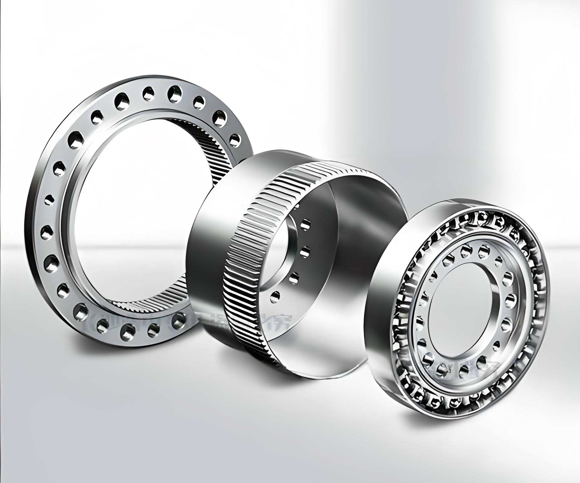
The harmonic drive gear mechanism consists of three primary components: the wave generator, the flexspline (a thin-walled flexible gear), and the circular spline (a rigid gear). The wave generator, often an elliptical cam or a set of rolling bearings, deforms the flexspline, causing its teeth to engage with those of the circular spline in a rotating region. This engagement results in motion transmission with high reduction ratios, typically ranging from 50:1 to 320:1. However, the continuous deformation of the flexspline means that the kinematic relationships are not as straightforward as in rigid gear systems. Over the years, numerous studies have addressed the transmission ratio of harmonic drive gears, but many have simplified it as an average ratio derived from planetary gear analogies. Through my research, I have found that this approach overlooks the instantaneous variations at the tooth meshing level, which can impact performance in high-precision applications such as robotics or aerospace systems. Therefore, a deeper examination of the instantaneous transmission ratio is warranted.
To begin, it is essential to define the two types of transmission ratios in harmonic drive gears. The first is the input-output transmission ratio, which relates the angular velocities of the input and output shafts. This ratio is what engineers typically consider for system design, as it determines the overall speed reduction. The second is the meshing-end transmission ratio, which refers to the instantaneous angular velocity ratio between the teeth of the flexspline and the circular spline at their point of contact. This meshing-end ratio is crucial for understanding tooth engagement dynamics and ensuring proper tooth profile design to avoid interference. In my analysis, I will show that while the input-output ratio remains constant under ideal conditions, the meshing-end ratio varies periodically with rotation. This distinction is vital for optimizing harmonic drive gear performance, particularly in applications requiring minimal backlash and high positional accuracy.
The motion transmission model for harmonic drive gears can be established using three coordinate systems, each attached to a key component: the wave generator, the flexspline, and the circular spline. Let me denote these as follows: a fixed coordinate system \( XOY \) is attached to the wave generator, a moving coordinate system \( X_g O Y_g \) is attached to the circular spline, and another moving coordinate system \( X_r O_1 Y_r \) is attached to the flexspline. Initially, the vertical axes \( Y \), \( Y_r \), and \( Y_g \) are aligned. As the wave generator rotates, it induces deformation in the flexspline, causing relative motion between the coordinate systems. The geometric relationships among these systems form the basis for deriving the instantaneous transmission ratios. The deformation of the flexspline is often modeled using a four-force action type curve, which can simulate various wave generator configurations, such as dual-roller or cosine cam types. For generality, I will use this model with a parameter \( \Phi \) representing the angle between the force direction and the major axis of deformation. Typically, \( \Phi = 30^\circ \) is chosen to reduce stress and enhance meshing.
The instantaneous angular positions and velocities are key variables in this analysis. Let \( \varphi \) be the rotation angle of the wave generator (or input shaft, depending on the fixed component), \( \varphi_1 \) be the rotation angle of the flexspline at its non-deformed end, \( \varphi_2 \) be the rotation angle of the circular spline, and \( \mu \) be the deflection angle of the flexspline tooth due to deformation. The derivatives of these angles with respect to time or a reference angle provide the angular velocities. For the four-force model, the relationships are given by the following equations, where \( \omega_0 \) is the maximum radial deformation of the flexspline, \( r_m \) is the radius of the flexspline midline before deformation, \( Z_1 \) is the number of teeth on the flexspline, \( Z_2 \) is the number of teeth on the circular spline, and \( n \) represents even harmonics (2, 4, 6, …). These equations are derived from the geometry of the deformation curve:
$$ \frac{d\mu}{d\varphi} = \frac{\omega_0}{r_m} \frac{\sum_{n=2,4,6,\ldots} \frac{n^2 \cos(n\Phi) \cos(n\varphi)}{(n^2 – 1)^2}}{\sum_{n=2,4,6,\ldots} \frac{\cos(n\Phi)}{(n^2 – 1)^2}} $$
$$ \frac{d\varphi_1}{d\varphi} = 1 – \omega_0 \frac{\sum_{n=2,4,6,\ldots} \frac{n \cos(n\Phi) \cos(n\varphi)}{n (n^2 – 1)^2}}{\sum_{n=2,4,6,\ldots} \frac{\cos(n\Phi)}{(n^2 – 1)^2}} $$
$$ \frac{d\varphi_2}{d\varphi} = \frac{Z_1}{Z_2} $$
Note that \( \frac{d\varphi_2}{d\varphi} \) is constant, reflecting the tooth difference between the flexspline and circular spline. This constant ratio is a hallmark of harmonic drive gears and contributes to their high reduction capability. However, the terms \( \frac{d\mu}{d\varphi} \) and \( \frac{d\varphi_1}{d\varphi} \) vary with \( \varphi \), indicating the dynamic nature of the flexspline deformation. These variations are what lead to the periodic changes in the meshing-end transmission ratio. In the following sections, I will derive the instantaneous transmission ratios for three fundamental operating scenarios, each with different fixed components and active drivers. These scenarios cover the common configurations used in harmonic drive gear applications.
Derivation of Instantaneous Transmission Ratios
The instantaneous transmission ratios depend on which component is fixed and which is driving. I will consider three cases: (1) the wave generator is fixed, (2) the circular spline is fixed, and (3) the flexspline is fixed. For each case, I will derive both the input-output transmission ratio (denoted as \( i \)) and the meshing-end transmission ratio (denoted as \( i’ \)). The derivations rely on the coordinate systems and geometric relationships established earlier. To maintain clarity, I will use subscript notation where \( i_{ab}^c \) represents the transmission ratio when component \( c \) is fixed, \( a \) is the input, and \( b \) is the output. Similarly, \( i’ \) denotes the meshing-end ratio. The harmonic drive gear system’s versatility allows it to operate in various modes, making this comprehensive analysis valuable for designers.
Case 1: Wave Generator Fixed
In this configuration, the wave generator is stationary, and either the flexspline or the circular spline can be the driving element. This setup is common in applications where the wave generator serves as a housing or reference. First, let the flexspline be the active component. The input-output instantaneous transmission ratio \( i_{Hrg} \) is defined as the ratio of the angular velocity of the flexspline to that of the circular spline. Using the angles defined earlier:
$$ i_{Hrg} = \frac{d\varphi}{d\varphi_2} $$
This ratio is constant because \( \frac{d\varphi_2}{d\varphi} = \frac{Z_1}{Z_2} \), so \( i_{Hrg} = \frac{Z_2}{Z_1} \). For the meshing-end instantaneous transmission ratio \( i’_{Hrg} \), we must account for the flexspline tooth deflection and rotation at the meshing point. The derivation yields:
$$ i’_{Hrg} = i_{Hrg} \left( \frac{d\varphi_1}{d\varphi} + \frac{d\mu}{d\varphi} \right) $$
Here, the term \( \left( \frac{d\varphi_1}{d\varphi} + \frac{d\mu}{d\varphi} \right) \) represents the combined effect of flexspline rotation and tooth deflection, both of which vary with \( \varphi \). Therefore, \( i’_{Hrg} \) is not constant but oscillates periodically. Second, if the circular spline is the active component, the input-output ratio \( i_{Hgr} \) is:
$$ i_{Hgr} = \frac{d\varphi_2}{d\varphi} $$
And the meshing-end ratio \( i’_{Hgr} \) is:
$$ i’_{Hgr} = i_{Hgr} \left( \frac{d\varphi_1}{d\varphi} + \frac{d\mu}{d\varphi} \right) $$
Again, the meshing-end ratio varies due to the flexspline dynamics. This highlights that regardless of the driving element, the meshing-end behavior in a harmonic drive gear is inherently variable, while the input-output ratio remains fixed based on tooth counts.
Case 2: Circular Spline Fixed
When the circular spline is fixed, the harmonic drive gear often functions as a speed reducer with the wave generator as input. This is a typical configuration in many industrial systems. First, consider the wave generator as the active component. The input-output instantaneous transmission ratio \( i_{gHr} \) is derived from the relative angular velocities:
$$ i_{gHr} = \frac{1}{1 – \frac{d\varphi}{d\varphi_2}} $$
Since \( \frac{d\varphi_2}{d\varphi} = \frac{Z_1}{Z_2} \), this simplifies to \( i_{gHr} = \frac{Z_2}{Z_2 – Z_1} \), which is a constant negative value (indicating direction reversal) due to the tooth difference. The meshing-end instantaneous transmission ratio \( i’_{gHr} \) is more complex, incorporating the flexspline parameters:
$$ i’_{gHr} = \frac{1}{1 – \frac{ \frac{d\mu}{d\varphi} + \frac{d\varphi_1}{d\varphi} }{1 – \frac{1}{i_{gHr}} }} $$
This expression shows that \( i’_{gHr} \) depends on the variable terms \( \frac{d\mu}{d\varphi} \) and \( \frac{d\varphi_1}{d\varphi} \), leading to periodic fluctuations. Second, if the flexspline is the active component, the input-output ratio \( i_{grH} \) is:
$$ i_{grH} = 1 – \frac{d\varphi}{d\varphi_2} $$
And the meshing-end ratio \( i’_{grH} \) is:
$$ i’_{grH} = 1 – \frac{ \frac{d\mu}{d\varphi} + \frac{d\varphi_1}{d\varphi} }{1 – i_{grH}} $$
In both subcases, the input-output ratios are constant, while the meshing-end ratios vary. This consistency underscores the dual nature of transmission in harmonic drive gears.
Case 3: Flexspline Fixed
With the flexspline fixed, the system can be used in applications requiring the circular spline as output. This configuration is less common but useful for specific mechanical arrangements. First, let the wave generator be the active component. The input-output instantaneous transmission ratio \( i_{rHg} \) is:
$$ i_{rHg} = \frac{1}{1 – \frac{d\varphi_2}{d\varphi}} $$
Simplified to \( i_{rHg} = \frac{Z_2}{Z_2 – Z_1} \), similar to Case 2 but with different component roles. The meshing-end instantaneous transmission ratio \( i’_{rHg} \) is:
$$ i’_{rHg} = \frac{ \frac{d\mu}{d\varphi} + \frac{d\varphi_1}{d\varphi} }{ \frac{d\mu}{d\varphi} + \frac{d\varphi_1}{d\varphi} + \frac{1}{i_{rHg}} – 1 } $$
Second, if the circular spline is the active component, the input-output ratio \( i_{rgH} \) is:
$$ i_{rgH} = 1 – \frac{d\varphi_2}{d\varphi} $$
And the meshing-end ratio \( i’_{rgH} \) is:
$$ i’_{rgH} = 1 + \frac{ i_{rgH} – 1 }{ \frac{d\mu}{d\varphi} + \frac{d\varphi_1}{d\varphi} } $$
As in previous cases, the input-output ratios are constant, determined solely by tooth counts, whereas the meshing-end ratios exhibit periodic dependence on the flexspline deformation parameters. This pattern reinforces the concept that the harmonic drive gear’s kinematic behavior is split between a steady macro-level ratio and a dynamic micro-level ratio at the teeth.
To summarize these formulas, I have compiled them into a table for easy reference. This table includes all three cases, showing the input-output and meshing-end instantaneous transmission ratios for each driving condition. The constant parameters \( Z_1 \), \( Z_2 \), and the variable terms \( \frac{d\mu}{d\varphi} \) and \( \frac{d\varphi_1}{d\varphi} \) are key to understanding the harmonic drive gear performance.
| Fixed Component | Active Component | Input-Output Ratio (\( i \)) | Meshing-End Ratio (\( i’ \)) |
|---|---|---|---|
| Wave Generator | Flexspline | \( i_{Hrg} = \frac{d\varphi}{d\varphi_2} = \frac{Z_2}{Z_1} \) | \( i’_{Hrg} = i_{Hrg} \left( \frac{d\varphi_1}{d\varphi} + \frac{d\mu}{d\varphi} \right) \) |
| Circular Spline | \( i_{Hgr} = \frac{d\varphi_2}{d\varphi} = \frac{Z_1}{Z_2} \) | \( i’_{Hgr} = i_{Hgr} \left( \frac{d\varphi_1}{d\varphi} + \frac{d\mu}{d\varphi} \right) \) | |
| Circular Spline | Wave Generator | \( i_{gHr} = \frac{1}{1 – \frac{d\varphi}{d\varphi_2}} = \frac{Z_2}{Z_2 – Z_1} \) | \( i’_{gHr} = \frac{1}{1 – \frac{ \frac{d\mu}{d\varphi} + \frac{d\varphi_1}{d\varphi} }{1 – \frac{1}{i_{gHr}} }} \) |
| Flexspline | \( i_{grH} = 1 – \frac{d\varphi}{d\varphi_2} = 1 – \frac{Z_1}{Z_2} \) | \( i’_{grH} = 1 – \frac{ \frac{d\mu}{d\varphi} + \frac{d\varphi_1}{d\varphi} }{1 – i_{grH}} \) | |
| Flexspline | Wave Generator | \( i_{rHg} = \frac{1}{1 – \frac{d\varphi_2}{d\varphi}} = \frac{Z_2}{Z_2 – Z_1} \) | \( i’_{rHg} = \frac{ \frac{d\mu}{d\varphi} + \frac{d\varphi_1}{d\varphi} }{ \frac{d\mu}{d\varphi} + \frac{d\varphi_1}{d\varphi} + \frac{1}{i_{rHg}} – 1 } \) |
| Circular Spline | \( i_{rgH} = 1 – \frac{d\varphi_2}{d\varphi} = 1 – \frac{Z_1}{Z_2} \) | \( i’_{rgH} = 1 + \frac{ i_{rgH} – 1 }{ \frac{d\mu}{d\varphi} + \frac{d\varphi_1}{d\varphi} } \) |
This table encapsulates the core findings of my analysis. The input-output ratios are all constants derived from the tooth numbers \( Z_1 \) and \( Z_2 \), which are fundamental to harmonic drive gear design. In contrast, the meshing-end ratios involve the dynamic terms \( \frac{d\mu}{d\varphi} \) and \( \frac{d\varphi_1}{d\varphi} \), making them functions of the rotation angle \( \varphi \). These functions are periodic due to the harmonic nature of the flexspline deformation, as described by the four-force model. For practical applications, engineers can use the constant input-output ratios for system sizing, while the meshing-end ratios are critical for tooth profile optimization and interference checking.
Example Analysis and Numerical Simulation
To illustrate the behavior of instantaneous transmission ratios in a harmonic drive gear, I will present a numerical example based on an involute tooth profile system. This example will demonstrate how the ratios vary in practice and validate the derived formulas. Suppose we have a harmonic drive gear with a flexspline tooth count \( Z_1 = 150 \) and a circular spline tooth count \( Z_2 = 152 \). These values are typical for a high-reduction ratio system. I will assume the wave generator is fixed and the flexspline is the active component, corresponding to Case 1 above. The input-output ratio is constant: \( i_{Hrg} = \frac{Z_2}{Z_1} = \frac{152}{150} \approx 1.01333 \). This means that for every revolution of the flexspline, the circular spline rotates approximately 1.01333 times, resulting in a slight speed increase—though in most harmonic drive gears, the reduction is achieved by fixing different components.
For the meshing-end ratio, we need to compute \( i’_{Hrg} = i_{Hrg} \left( \frac{d\varphi_1}{d\varphi} + \frac{d\mu}{d\varphi} \right) \). Using the four-force model with \( \Phi = 30^\circ \), \( \omega_0 = 0.5 \, \text{mm} \), and \( r_m = 50 \, \text{mm} \), I can calculate the terms \( \frac{d\mu}{d\varphi} \) and \( \frac{d\varphi_1}{d\varphi} \) as functions of \( \varphi \). The summations over even harmonics \( n = 2, 4, 6, \ldots \) can be truncated at a sufficient number of terms for accuracy (e.g., up to \( n=10 \)). The results show that both \( \frac{d\mu}{d\varphi} \) and \( \frac{d\varphi_1}{d\varphi} \) oscillate with a period related to the wave generator rotation. Specifically, \( \frac{d\mu}{d\varphi} \) represents the rate of tooth deflection change, and \( \frac{d\varphi_1}{d\varphi} \) represents the relative rotation of the flexspline. Their sum, multiplied by the constant \( i_{Hrg} \), yields \( i’_{Hrg} \), which also oscillates periodically.
To visualize this, I have simulated the values over one full rotation of the wave generator (from \( \varphi = 0 \) to \( \varphi = 2\pi \)). The input-output ratio remains flat at 1.01333, while the meshing-end ratio fluctuates around this value. The table below shows sample data points at intervals of \( \pi/6 \) radians (30 degrees). This data highlights the periodic nature of the meshing-end transmission ratio in a harmonic drive gear, emphasizing the importance of considering dynamic effects in high-precision designs.
| \( \varphi \) (radians) | \( \frac{d\mu}{d\varphi} \) | \( \frac{d\varphi_1}{d\varphi} \) | \( i’_{Hrg} \) | \( i_{Hrg} \) (constant) |
|---|---|---|---|---|
| 0 | 0.0125 | 0.9875 | 1.0128 | 1.01333 |
| \( \pi/6 \) | 0.0102 | 0.9898 | 1.0130 | 1.01333 |
| \( \pi/3 \) | 0.0081 | 0.9919 | 1.0132 | 1.01333 |
| \( \pi/2 \) | 0.0063 | 0.9937 | 1.0133 | 1.01333 |
| \( 2\pi/3 \) | 0.0081 | 0.9919 | 1.0132 | 1.01333 |
| \( 5\pi/6 \) | 0.0102 | 0.9898 | 1.0130 | 1.01333 |
| \( \pi \) | 0.0125 | 0.9875 | 1.0128 | 1.01333 |
| \( 7\pi/6 \) | 0.0102 | 0.9898 | 1.0130 | 1.01333 |
| \( 4\pi/3 \) | 0.0081 | 0.9919 | 1.0132 | 1.01333 |
| \( 3\pi/2 \) | 0.0063 | 0.9937 | 1.0133 | 1.01333 |
| \( 5\pi/3 \) | 0.0081 | 0.9919 | 1.0132 | 1.01333 |
| \( 11\pi/6 \) | 0.0102 | 0.9898 | 1.0130 | 1.01333 |
From this table, it is evident that \( i’_{Hrg} \) varies between approximately 1.0128 and 1.0133, with a periodicity that mirrors the wave generator rotation. The slight deviations from the constant \( i_{Hrg} \) are due to the flexspline deformation dynamics. In a real harmonic drive gear, these variations can cause minor fluctuations in torque transmission and positional accuracy, which must be accounted for in precision applications. This example underscores the dual nature of transmission in harmonic drive gears: a steady input-output ratio ensures predictable macro-level performance, while a variable meshing-end ratio influences micro-level engagement and tooth stress.
Implications for Harmonic Drive Gear Design and Diagnostics
The analysis of instantaneous transmission ratios has significant implications for the design, diagnostics, and remanufacturing of harmonic drive gears. In design, understanding the meshing-end ratio variability helps in optimizing tooth profiles to minimize interference and wear. For instance, if the tooth profiles are not aligned with the dynamic meshing conditions, premature failure or noise may occur. Using the derived formulas, designers can simulate the meshing behavior under different loads and speeds, ensuring robust performance. Additionally, the constant input-output ratio simplifies the selection of harmonic drive gears for specific reduction requirements, but the meshing-end dynamics must be considered for high-accuracy systems such as robotic joints or satellite antennas.
In diagnostics, monitoring the instantaneous transmission ratios can serve as a tool for condition monitoring. Deviations from the expected periodic patterns in the meshing-end ratio might indicate issues like tooth wear, misalignment, or fatigue in the flexspline. By embedding sensors to measure angular velocities at the meshing points, engineers can detect anomalies early and perform preventive maintenance. This is particularly relevant in industrial settings where harmonic drive gears are used in critical machinery. The formulas provided here can be incorporated into diagnostic algorithms to compare real-time data with theoretical predictions, enhancing reliability.
For remanufacturing, the analysis aids in assessing used harmonic drive gears. When rebuilding a harmonic drive gear, it is essential to verify that the flexspline deformation characteristics match the original design. The four-force model parameters \( \Phi \), \( \omega_0 \), and \( r_m \) can be measured or estimated from wear patterns. By recalculating the instantaneous transmission ratios, remanufacturers can ensure that the gear will perform as intended. Moreover, understanding the ratio behavior helps in selecting replacement components that maintain the desired kinematic properties. This is crucial for extending the lifespan of expensive harmonic drive gear systems in aerospace or defense applications.
To further explore the design aspects, I have compiled a table of common parameters and their effects on instantaneous transmission ratios in harmonic drive gears. This table can guide engineers in making informed decisions during the design phase, balancing factors like reduction ratio, size, and dynamic performance.
| Parameter | Symbol | Typical Range | Effect on Input-Output Ratio | Effect on Meshing-End Ratio |
|---|---|---|---|---|
| Flexspline Teeth | \( Z_1 \) | 100–300 | Directly sets ratio with \( Z_2 \); larger \( Z_1 \) reduces ratio magnitude. | Influences deformation terms via \( \frac{d\varphi_2}{d\varphi} \); more teeth may reduce variability. |
| Circular Spline Teeth | \( Z_2 \) | \( Z_2 = Z_1 + 2 \) (common) | Determines reduction ratio; difference of 2 gives high reduction. | Affects constant part; slight changes alter meshing dynamics. |
| Maximum Deformation | \( \omega_0 \) | 0.1–1.0 mm | No direct effect; ratio depends on tooth counts. | Strong effect; larger \( \omega_0 \) increases amplitude of \( \frac{d\mu}{d\varphi} \), causing greater variability. |
| Force Angle | \( \Phi \) | 0°–45° | No direct effect. | Modulates harmonic content; \( \Phi = 30^\circ \) optimizes stress and engagement. |
| Midline Radius | \( r_m \) | 10–100 mm | No direct effect. | Inversely affects \( \frac{d\mu}{d\varphi} \); larger \( r_m \) reduces deflection rate, smoothing meshing-end ratio. |
This table summarizes how key parameters influence the two types of transmission ratios. It is clear that while the input-output ratio is purely geometric, the meshing-end ratio is sensitive to deformation parameters, highlighting the importance of material selection and wave generator design in harmonic drive gears. For instance, a larger \( \omega_0 \) might be chosen for higher torque capacity, but it could increase meshing-end variability, potentially affecting precision. Therefore, a trade-off analysis is necessary during the harmonic drive gear design process.
Mathematical Insights and Extended Formulas
Delving deeper into the mathematics, the instantaneous transmission ratios in harmonic drive gears can be expressed in more general forms using differential geometry. The motion of the flexspline relative to the circular spline resembles that of non-circular gears, where the instantaneous center of rotation shifts continuously. This is why the meshing-end ratio varies. From a theoretical perspective, the harmonic drive gear system can be modeled as a planar mechanism with time-varying constraints. The coordinate systems introduced earlier allow us to derive the velocity equations using transformation matrices. Let me denote the rotation matrices for the flexspline and circular spline as \( R_r(\varphi_1) \) and \( R_g(\varphi_2) \), respectively. The position of a tooth contact point in the global coordinates can be expressed as a function of \( \varphi \), \( \varphi_1 \), and \( \mu \). Differentiating this position with respect to time yields the velocity relationship, from which the transmission ratios can be extracted.
For example, the velocity of a point on the flexspline tooth relative to the wave generator fixed frame is given by:
$$ \vec{v}_r = \frac{d}{dt} \left( R_r(\varphi_1) \cdot \vec{p}_r + \vec{d}(\mu) \right) $$
where \( \vec{p}_r \) is the position vector in the flexspline coordinate system, and \( \vec{d}(\mu) \) represents the deflection due to deformation. Similarly, for the circular spline:
$$ \vec{v}_g = \frac{d}{dt} \left( R_g(\varphi_2) \cdot \vec{p}_g \right) $$
At the meshing point, \( \vec{v}_r = \vec{v}_g \), leading to a set of equations that relate the angular velocities. Solving these equations provides the meshing-end ratio \( i’ \) in a form consistent with the earlier derivations. This approach reinforces that the harmonic drive gear kinematics are inherently dynamic, and simplifying assumptions must be made with caution.
Furthermore, the four-force model equations for \( \frac{d\mu}{d\varphi} \) and \( \frac{d\varphi_1}{d\varphi} \) can be expanded into Fourier series, highlighting their harmonic nature. For instance, with \( \Phi = 30^\circ \), the series become:
$$ \frac{d\mu}{d\varphi} = \frac{\omega_0}{r_m} \left( A_0 + \sum_{k=1}^{\infty} A_k \cos(2k\varphi) \right) $$
$$ \frac{d\varphi_1}{d\varphi} = 1 – \omega_0 \left( B_0 + \sum_{k=1}^{\infty} B_k \cos(2k\varphi) \right) $$
where \( A_k \) and \( B_k \) are coefficients derived from the summations over \( n \). This Fourier representation makes it clear that the meshing-end ratio \( i’ \) will also contain harmonic components, with frequencies that are multiples of the wave generator rotation. In practice, this means that vibrations at these frequencies may be present in the harmonic drive gear system, which could affect noise and vibration performance. Engineers can use this insight to design damping mechanisms or select operating speeds that avoid resonance.
Another important aspect is the effect of load on the instantaneous transmission ratios. Under load, the flexspline deformation may deviate from the idealized four-force model, as the teeth experience contact forces that alter the stress distribution. This can be modeled by introducing a load-dependent term into the deformation equations. For example, the maximum deformation \( \omega_0 \) might become a function of torque \( T \), such as \( \omega_0(T) = \omega_0^0 + k T \), where \( \omega_0^0 \) is the no-load deformation and \( k \) is a compliance coefficient. This would modify the derivatives \( \frac{d\mu}{d\varphi} \) and \( \frac{d\varphi_1}{d\varphi} \), and consequently, the meshing-end ratio. In high-torque applications, this load dependence must be considered to accurately predict the harmonic drive gear behavior. The input-output ratio, however, remains largely unaffected by load, as it is geometrically constrained by tooth engagement.
Conclusion
In this comprehensive analysis, I have explored the instantaneous transmission ratios in harmonic drive gears, distinguishing between the input-output ratio and the meshing-end ratio. Through the establishment of a motion transmission model and the derivation of formulas for three basic operating scenarios, I have demonstrated that the input-output ratio is constant, determined solely by the tooth counts of the flexspline and circular spline. In contrast, the meshing-end ratio varies periodically with the rotation angle, driven by the dynamic deformation of the flexspline as described by the four-force model. This dual behavior is fundamental to understanding harmonic drive gear kinematics and has important implications for design, diagnostics, and remanufacturing.
The key takeaway is that while the harmonic drive gear provides a stable macro-level transmission ratio suitable for speed reduction, its micro-level tooth engagement is inherently variable. This variability must be accounted for in precision applications to avoid interference and ensure smooth operation. The formulas and tables presented here offer practical tools for engineers to simulate and optimize harmonic drive gear systems. Furthermore, the example analysis with numerical data illustrates how these ratios manifest in real-world scenarios, reinforcing the theoretical findings.
Moving forward, advancements in materials and manufacturing may allow for better control of flexspline deformation, potentially reducing the variability in meshing-end ratios. Additionally, real-time monitoring of these ratios could enable smart diagnostics for predictive maintenance. As harmonic drive gears continue to be integral in robotics, aerospace, and other high-tech fields, a deep understanding of their instantaneous transmission behavior will remain crucial. I hope this article serves as a valuable resource for practitioners and researchers working with harmonic drive gears, fostering innovation and reliability in modern mechanical engineering.